

Appendix J
J.1 Integral Algorithm for Colored Noise Simulation
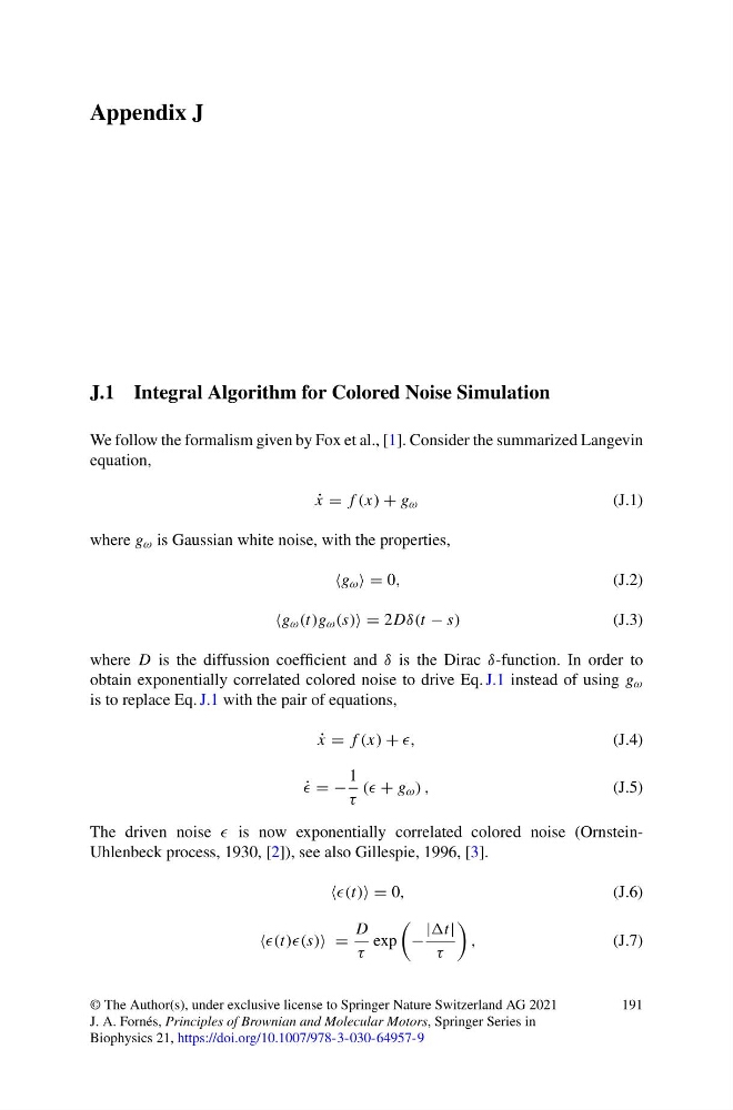
We follow the formalism given by Fox et al., [1]. Consider the summarized Langevin
equation,
˙
x = f (x) + g ω
(J.1)
where g ω is Gaussian white noise, with the properties,
g ω = 0,
(J.2)
g ω (t)g ω (s) = 2Dδ(t − s)
(J.3)
where D is the diffussion coefficient and δ is the Dirac δ-function. In order to
obtain exponentially correlated colored noise to drive Eq. J.1 instead of using g ω
is to replace Eq. J.1 with the pair of equations,
˙
x = f (x) + ,
(J.4)
˙
= −
1
τ
( + g ω ) ,
(J.5)
The driven noise is now exponentially correlated colored noise (OrnsteinUhlenbeck process, 1930, [2]), see also Gillespie, 1996, [3].
= 0,
(J.6)
(t))(s) =
D
τ
exp
−
|t|
τ
,
(J.7)
© The Author(s), under exclusive license to Springer Nature Switzerland AG 2021
J. A. Fornés, Principles of Brownian and Molecular Motors, Springer Series in
Biophysics 21, https://doi.org/10.1007/978-3-030-64957-9
191
J.1 Integral Algorithm for Colored Noise Simulation
We follow the formalism given by Fox et al., [1]. Consider the summarized Langevin
equation,
˙
x = f (x) + g ω
(J.1)
where g ω is Gaussian white noise, with the properties,
g ω = 0,
(J.2)
g ω (t)g ω (s) = 2Dδ(t − s)
(J.3)
where D is the diffussion coefficient and δ is the Dirac δ-function. In order to
obtain exponentially correlated colored noise to drive Eq. J.1 instead of using g ω
is to replace Eq. J.1 with the pair of equations,
˙
x = f (x) + ,
(J.4)
˙
= −
1
τ
( + g ω ) ,
(J.5)
The driven noise is now exponentially correlated colored noise (OrnsteinUhlenbeck process, 1930, [2]), see also Gillespie, 1996, [3].
= 0,
(J.6)
(t))(s) =
D
τ
exp
−
|t|
τ
,
(J.7)
© The Author(s), under exclusive license to Springer Nature Switzerland AG 2021
J. A. Fornés, Principles of Brownian and Molecular Motors, Springer Series in
Biophysics 21, https://doi.org/10.1007/978-3-030-64957-9
191