

176
Appendix F
dE k
dt
=
1
2
d
p 2
dt
(F.7)
Then we need to calculate d
p 2
, namely
d
p
2
= (p + dp)
2
− p
2
= (dp)
2
+ 2pdp
(F.8)
To finish our calculation, from Eq. F.5, we get (dp)
2
(dp)
2
= 2k B T
(F.9)
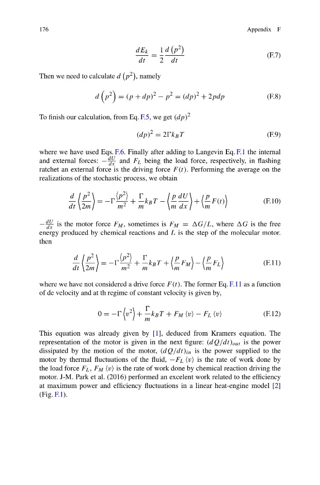
where we have used Eqs. F.6. Finally after adding to Langevin Eq. F.1 the internal
and external forces: −
dU
dx and F L being the load force, respectively, in flashing
ratchet an external force is the driving force F (t). Performing the average on the
realizations of the stochastic process, we obtain
d
dt
p 2
2m
= −
p 2
m 2 +
m
k B T −
p
m
dU
dx
+
p
m
F (t)
(F.10)
−
dU
dx is the motor force F M , sometimes is F M = where G is the free
energy produced by chemical reactions and L is the step of the molecular motor.
then
d
dt
p 2
2m
= −
p 2
m 2 +
m
k B T +
p
m
F M
−
p
m
F L
(F.11)
where we have not considered a drive force F (t). The former Eq. F.11 as a function
of de velocity and at th regime of constant velocity is given by,
0 = −
v
2
+
m
k B T + F M v − F L v
(F.12)
This equation was already given by [1], deduced from Kramers equation. The
representation of the motor is given in the next figure: (dQ/dt) out is the power
dissipated by the motion of the motor, (dQ/dt) in is the power supplied to the
motor by thermal fluctuations of the fluid, −F L v is the rate of work done by
the load force F L , F M v is the rate of work done by chemical reaction driving the
motor. J-M. Park et al. (2016) performed an excelent work related to the efficiency
at maximum power and efficiency fluctuations in a linear heat-engine model [2]
(Fig. F.1).
Appendix F
dE k
dt
=
1
2
d
p 2
dt
(F.7)
Then we need to calculate d
p 2
, namely
d
p
2
= (p + dp)
2
− p
2
= (dp)
2
+ 2pdp
(F.8)
To finish our calculation, from Eq. F.5, we get (dp)
2
(dp)
2
= 2k B T
(F.9)
where we have used Eqs. F.6. Finally after adding to Langevin Eq. F.1 the internal
and external forces: −
dU
dx and F L being the load force, respectively, in flashing
ratchet an external force is the driving force F (t). Performing the average on the
realizations of the stochastic process, we obtain
d
dt
p 2
2m
= −
p 2
m 2 +
m
k B T −
p
m
dU
dx
+
p
m
F (t)
(F.10)
−
dU
dx is the motor force F M , sometimes is F M = where G is the free
energy produced by chemical reactions and L is the step of the molecular motor.
then
d
dt
p 2
2m
= −
p 2
m 2 +
m
k B T +
p
m
F M
−
p
m
F L
(F.11)
where we have not considered a drive force F (t). The former Eq. F.11 as a function
of de velocity and at th regime of constant velocity is given by,
0 = −
v
2
+
m
k B T + F M v − F L v
(F.12)
This equation was already given by [1], deduced from Kramers equation. The
representation of the motor is given in the next figure: (dQ/dt) out is the power
dissipated by the motion of the motor, (dQ/dt) in is the power supplied to the
motor by thermal fluctuations of the fluid, −F L v is the rate of work done by
the load force F L , F M v is the rate of work done by chemical reaction driving the
motor. J-M. Park et al. (2016) performed an excelent work related to the efficiency
at maximum power and efficiency fluctuations in a linear heat-engine model [2]
(Fig. F.1).