

Appendix A
A.1 Master Equation
A.1.1 Transition Rate
Consider discrete states of a system S j , where j is an integer. Temporal change
among discrete states is called state transition. The so-called transition rate, ω i→j ,
from the discrete state S i to the discrete state S j is defined as follows:
• Suppose that a system is in the state S i at a time t.
• The (conditional) probability that the system makes the transition to a different
state S j during an infinitesimal time lapse, dt, is ω i→j dt.
A.1.2 Probability Flux
Consider a system in the state S i with the probability P i . Between S i and S j , there
is the flow of probability P j ω i→j from S i to S j and P i ω j →i from S j to S i . We call
the net flow to the probability per unit of time the (net) probability flux and denote
it by J i→j (=-J j →i ):
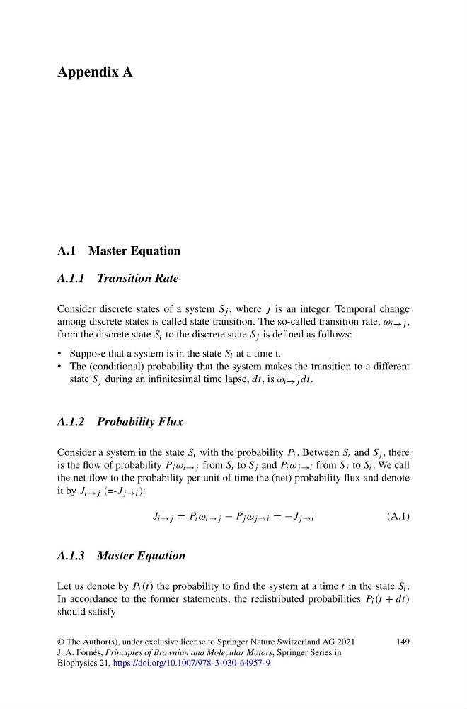
J i→j = P i ω i→j − P j ω j →i = −J j →i
(A.1)
A.1.3 Master Equation
Let us denote by P i (t) the probability to find the system at a time t in the state S i .
In accordance to the former statements, the redistributed probabilities P i (t + dt)
should satisfy
© The Author(s), under exclusive license to Springer Nature Switzerland AG 2021
J. A. Fornés, Principles of Brownian and Molecular Motors, Springer Series in
Biophysics 21, https://doi.org/10.1007/978-3-030-64957-9
149
A.1 Master Equation
A.1.1 Transition Rate
Consider discrete states of a system S j , where j is an integer. Temporal change
among discrete states is called state transition. The so-called transition rate, ω i→j ,
from the discrete state S i to the discrete state S j is defined as follows:
• Suppose that a system is in the state S i at a time t.
• The (conditional) probability that the system makes the transition to a different
state S j during an infinitesimal time lapse, dt, is ω i→j dt.
A.1.2 Probability Flux
Consider a system in the state S i with the probability P i . Between S i and S j , there
is the flow of probability P j ω i→j from S i to S j and P i ω j →i from S j to S i . We call
the net flow to the probability per unit of time the (net) probability flux and denote
it by J i→j (=-J j →i ):
J i→j = P i ω i→j − P j ω j →i = −J j →i
(A.1)
A.1.3 Master Equation
Let us denote by P i (t) the probability to find the system at a time t in the state S i .
In accordance to the former statements, the redistributed probabilities P i (t + dt)
should satisfy
© The Author(s), under exclusive license to Springer Nature Switzerland AG 2021
J. A. Fornés, Principles of Brownian and Molecular Motors, Springer Series in
Biophysics 21, https://doi.org/10.1007/978-3-030-64957-9
149