

8.1 The Quantum Langevin Equation
135
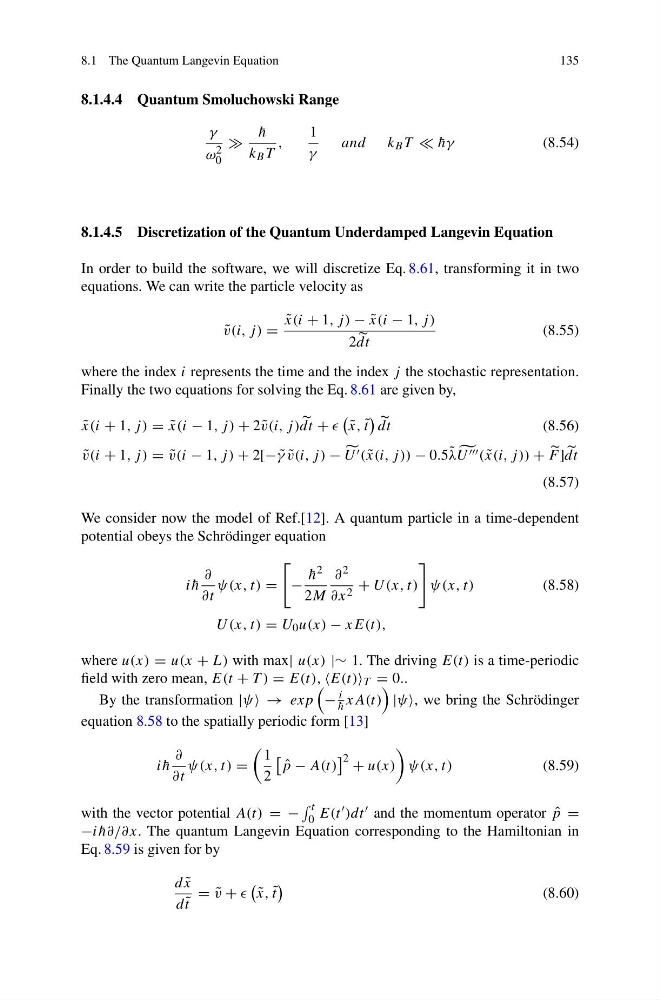
8.1.4.4 Quantum Smoluchowski Range
γ
ω 2
0
¯
h
k B T
,
1
γ
and k B T ¯
hγ
(8.54)
8.1.4.5 Discretization of the Quantum Underdamped Langevin Equation
In order to build the software, we will discretize Eq. 8.61, transforming it in two
equations. We can write the particle velocity as
˜
v(i, j ) =
˜
x(i + 1, j) − ˜
x(i − 1, j)
2
dt
(8.55)
where the index i represents the time and the index j the stochastic representation.
Finally the two equations for solving the Eq. 8.61 are given by,
˜
x(i + 1, j) = ˜
x(i − 1, j) + 2 ˜
v(i, j )
dt +
˜
x, ˜
t
dt
(8.56)
˜
v(i + 1, j) = ˜
v(i − 1, j) + 2[− ˜
γ ˜
v(i, j ) − U ( ˜
x(i, j )) − 0.5 ˜
λ
U ( ˜
x(i, j )) +
F ]
dt
(8.57)
We consider now the model of Ref.[12]. A quantum particle in a time-dependent
potential obeys the Schrödinger equation
i ¯
h
∂
∂t
ψ(x, t) =
−
¯
h 2
2M
∂ 2
∂x 2 + U(x, t)
ψ(x, t)
(8.58)
U(x, t) = U 0 u(x) − xE(t),
where u(x) = u(x + L) with max| u(x) |∼ 1. The driving E(t) is a time-periodic
field with zero mean, E(t + T ) = E(t), E(t) T = 0..
By the transformation |ψ → exp
−
i
¯
h xA(t)
|ψ, we bring the Schrödinger
equation 8.58 to the spatially periodic form [13]
i ¯
h
∂
∂t
ψ(x, t) =
1
2
ˆ
p − A(t)
2 + u(x)
ψ(x, t)
(8.59)
with the vector potential A(t) = −
t
0 E(t )dt and the momentum operator ˆ
p =
−i ¯
h∂/∂x. The quantum Langevin Equation corresponding to the Hamiltonian in
Eq. 8.59 is given for by
d ˜
x
d ˜
t
= ˜
v +
˜
x, ˜
t
(8.60)
135
8.1.4.4 Quantum Smoluchowski Range
γ
ω 2
0
¯
h
k B T
,
1
γ
and k B T ¯
hγ
(8.54)
8.1.4.5 Discretization of the Quantum Underdamped Langevin Equation
In order to build the software, we will discretize Eq. 8.61, transforming it in two
equations. We can write the particle velocity as
˜
v(i, j ) =
˜
x(i + 1, j) − ˜
x(i − 1, j)
2
dt
(8.55)
where the index i represents the time and the index j the stochastic representation.
Finally the two equations for solving the Eq. 8.61 are given by,
˜
x(i + 1, j) = ˜
x(i − 1, j) + 2 ˜
v(i, j )
dt +
˜
x, ˜
t
dt
(8.56)
˜
v(i + 1, j) = ˜
v(i − 1, j) + 2[− ˜
γ ˜
v(i, j ) − U ( ˜
x(i, j )) − 0.5 ˜
λ
U ( ˜
x(i, j )) +
F ]
dt
(8.57)
We consider now the model of Ref.[12]. A quantum particle in a time-dependent
potential obeys the Schrödinger equation
i ¯
h
∂
∂t
ψ(x, t) =
−
¯
h 2
2M
∂ 2
∂x 2 + U(x, t)
ψ(x, t)
(8.58)
U(x, t) = U 0 u(x) − xE(t),
where u(x) = u(x + L) with max| u(x) |∼ 1. The driving E(t) is a time-periodic
field with zero mean, E(t + T ) = E(t), E(t) T = 0..
By the transformation |ψ → exp
−
i
¯
h xA(t)
|ψ, we bring the Schrödinger
equation 8.58 to the spatially periodic form [13]
i ¯
h
∂
∂t
ψ(x, t) =
1
2
ˆ
p − A(t)
2 + u(x)
ψ(x, t)
(8.59)
with the vector potential A(t) = −
t
0 E(t )dt and the momentum operator ˆ
p =
−i ¯
h∂/∂x. The quantum Langevin Equation corresponding to the Hamiltonian in
Eq. 8.59 is given for by
d ˜
x
d ˜
t
= ˜
v +
˜
x, ˜
t
(8.60)