

66
3 Jet Substructure at the LHC
[GeV]
jet
T
p
20 30 40
2
10
2
10
×
2
3
10
3
10
×
2
Fractional JES uncertainty
0
0.02
0.04
0.06
0.08
0.1
ATLAS
in situ
= 0.4, EM+JES +
R
t
k
anti= 13 TeV
s
Data 2015,
= 0.0
η
Total uncertainty
JES
in situ
Absolute
JES
in situ
Relative
Flav. composition, unknown composition
Flav. response, unknown composition
Pile-up, average 2015 conditions
Punch-through, average 2015 conditions
(GeV)
T
p
20
100 200
1000
JEC uncertainty (%)
0
1
2
3
4
5
6
(8 TeV)
-1
19.7 fb
CMS
Total uncertainty
Excl. flavor, time
Absolute scale
Relative scale
=20)
〉
μ
〈
Pileup (
Jet flavor (QCD)
Time stability
R=0.5 PF+CHS
| = 0
jet
η
|
(8 TeV)
-1
19.7 fb
CMS
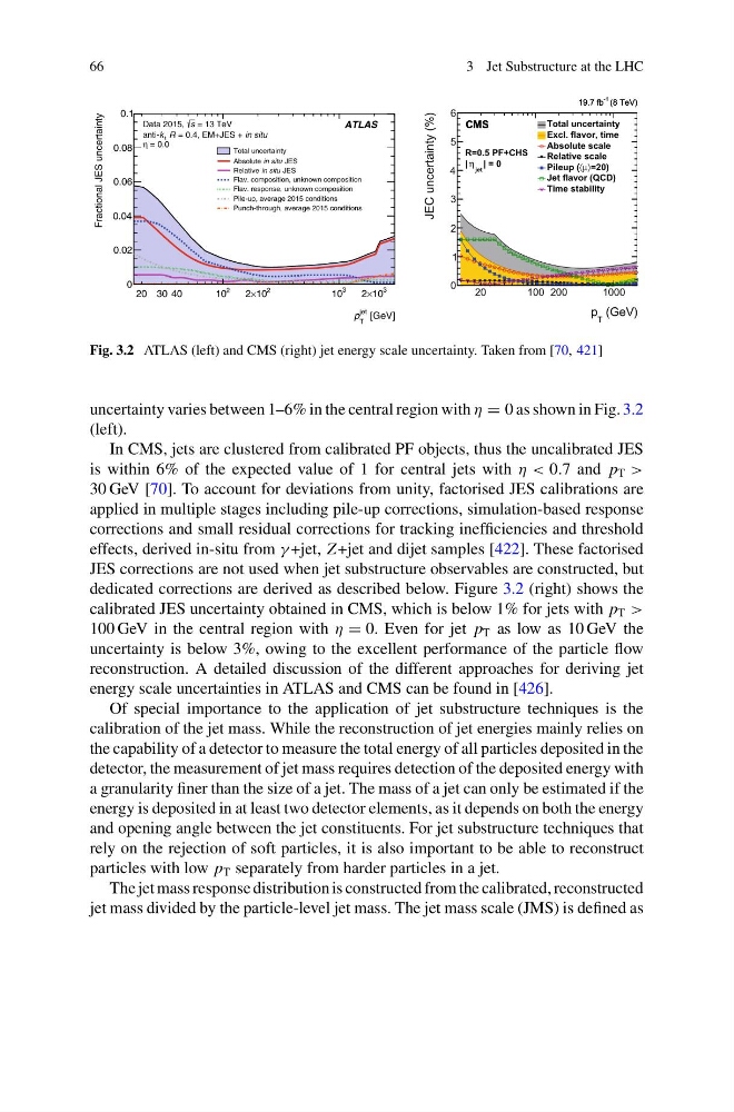
Fig. 3.2 ATLAS (left) and CMS (right) jet energy scale uncertainty. Taken from [70, 421]
uncertainty varies between 1–6% in the central region with η = 0 as shown in Fig. 3.2
(left).
In CMS, jets are clustered from calibrated PF objects, thus the uncalibrated JES
is within 6% of the expected value of 1 for central jets with η < 0.7 and p T >
30 GeV [70]. To account for deviations from unity, factorised JES calibrations are
applied in multiple stages including pile-up corrections, simulation-based response
corrections and small residual corrections for tracking inefficiencies and threshold
effects, derived in-situ from γ +jet, Z +jet and dijet samples [422]. These factorised
JES corrections are not used when jet substructure observables are constructed, but
dedicated corrections are derived as described below. Figure 3.2 (right) shows the
calibrated JES uncertainty obtained in CMS, which is below 1% for jets with p T >
100 GeV in the central region with η = 0. Even for jet p T as low as 10 GeV the
uncertainty is below 3%, owing to the excellent performance of the particle flow
reconstruction. A detailed discussion of the different approaches for deriving jet
energy scale uncertainties in ATLAS and CMS can be found in [426].
Of special importance to the application of jet substructure techniques is the
calibration of the jet mass. While the reconstruction of jet energies mainly relies on
the capability of a detector to measure the total energy of all particles deposited in the
detector, the measurement of jet mass requires detection of the deposited energy with
a granularity finer than the size of a jet. The mass of a jet can only be estimated if the
energy is deposited in at least two detector elements, as it depends on both the energy
and opening angle between the jet constituents. For jet substructure techniques that
rely on the rejection of soft particles, it is also important to be able to reconstruct
particles with low p T separately from harder particles in a jet.
The jet mass response distribution is constructed from the calibrated, reconstructed
jet mass divided by the particle-level jet mass. The jet mass scale (JMS) is defined as
3 Jet Substructure at the LHC
[GeV]
jet
T
p
20 30 40
2
10
2
10
×
2
3
10
3
10
×
2
Fractional JES uncertainty
0
0.02
0.04
0.06
0.08
0.1
ATLAS
in situ
= 0.4, EM+JES +
R
t
k
anti= 13 TeV
s
Data 2015,
= 0.0
η
Total uncertainty
JES
in situ
Absolute
JES
in situ
Relative
Flav. composition, unknown composition
Flav. response, unknown composition
Pile-up, average 2015 conditions
Punch-through, average 2015 conditions
(GeV)
T
p
20
100 200
1000
JEC uncertainty (%)
0
1
2
3
4
5
6
(8 TeV)
-1
19.7 fb
CMS
Total uncertainty
Excl. flavor, time
Absolute scale
Relative scale
=20)
〉
μ
〈
Pileup (
Jet flavor (QCD)
Time stability
R=0.5 PF+CHS
| = 0
jet
η
|
(8 TeV)
-1
19.7 fb
CMS
Fig. 3.2 ATLAS (left) and CMS (right) jet energy scale uncertainty. Taken from [70, 421]
uncertainty varies between 1–6% in the central region with η = 0 as shown in Fig. 3.2
(left).
In CMS, jets are clustered from calibrated PF objects, thus the uncalibrated JES
is within 6% of the expected value of 1 for central jets with η < 0.7 and p T >
30 GeV [70]. To account for deviations from unity, factorised JES calibrations are
applied in multiple stages including pile-up corrections, simulation-based response
corrections and small residual corrections for tracking inefficiencies and threshold
effects, derived in-situ from γ +jet, Z +jet and dijet samples [422]. These factorised
JES corrections are not used when jet substructure observables are constructed, but
dedicated corrections are derived as described below. Figure 3.2 (right) shows the
calibrated JES uncertainty obtained in CMS, which is below 1% for jets with p T >
100 GeV in the central region with η = 0. Even for jet p T as low as 10 GeV the
uncertainty is below 3%, owing to the excellent performance of the particle flow
reconstruction. A detailed discussion of the different approaches for deriving jet
energy scale uncertainties in ATLAS and CMS can be found in [426].
Of special importance to the application of jet substructure techniques is the
calibration of the jet mass. While the reconstruction of jet energies mainly relies on
the capability of a detector to measure the total energy of all particles deposited in the
detector, the measurement of jet mass requires detection of the deposited energy with
a granularity finer than the size of a jet. The mass of a jet can only be estimated if the
energy is deposited in at least two detector elements, as it depends on both the energy
and opening angle between the jet constituents. For jet substructure techniques that
rely on the rejection of soft particles, it is also important to be able to reconstruct
particles with low p T separately from harder particles in a jet.
The jet mass response distribution is constructed from the calibrated, reconstructed
jet mass divided by the particle-level jet mass. The jet mass scale (JMS) is defined as