

36
2 Phenomenology of Jet Substructure
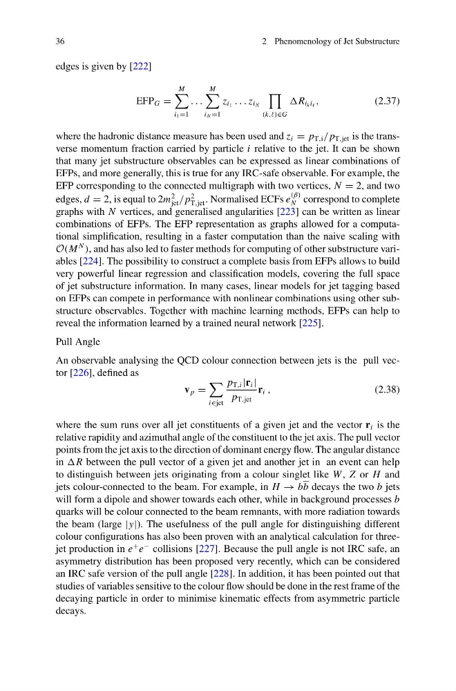
edges is given by [222]
EFP G =
M
i 1 =1
. . .
M
i N =1
z i 1 . . . z i N
(k,,)∈G
R i k i ,
(2.37)
where the hadronic distance measure has been used and z i = p T,i / p T,jet is the transverse momentum fraction carried by particle i relative to the jet. It can be shown
that many jet substructure observables can be expressed as linear combinations of
EFPs, and more generally, this is true for any IRC-safe observable. For example, the
EFP corresponding to the connected multigraph with two vertices, N = 2, and two
edges, d = 2, is equal to 2m
2
jet / p
2
T,jet . Normalised ECFs e
(β)
N correspond to complete
graphs with N vertices, and generalised angularities [223] can be written as linear
combinations of EFPs. The EFP representation as graphs allowed for a computational simplification, resulting in a faster computation than the naive scaling with
O(M
N
), and has also led to faster methods for computing of other substructure variables [224]. The possibility to construct a complete basis from EFPs allows to build
very powerful linear regression and classification models, covering the full space
of jet substructure information. In many cases, linear models for jet tagging based
on EFPs can compete in performance with nonlinear combinations using other substructure observables. Together with machine learning methods, EFPs can help to
reveal the information learned by a trained neural network [225].
Pull Angle
An observable analysing the QCD colour connection between jets is the pull vector [226], defined as
v p =
i∈jet
p T,i |r i |
p T,jet
r i ,
(2.38)
where the sum runs over all jet constituents of a given jet and the vector r i is the
relative rapidity and azimuthal angle of the constituent to the jet axis. The pull vector
points from the jet axis to the direction of dominant energy flow. The angular distance
in R between the pull vector of a given jet and another jet in an event can help
to distinguish between jets originating from a colour singlet like W , Z or H and
jets colour-connected to the beam. For example, in H → bb decays the two b jets
will form a dipole and shower towards each other, while in background processes b
quarks will be colour connected to the beam remnants, with more radiation towards
the beam (large |y|). The usefulness of the pull angle for distinguishing different
colour configurations has also been proven with an analytical calculation for threejet production in e
+ e
− collisions [227]. Because the pull angle is not IRC safe, an
asymmetry distribution has been proposed very recently, which can be considered
an IRC safe version of the pull angle [228]. In addition, it has been pointed out that
studies of variables sensitive to the colour flow should be done in the rest frame of the
decaying particle in order to minimise kinematic effects from asymmetric particle
decays.
2 Phenomenology of Jet Substructure
edges is given by [222]
EFP G =
M
i 1 =1
. . .
M
i N =1
z i 1 . . . z i N
(k,,)∈G
R i k i ,
(2.37)
where the hadronic distance measure has been used and z i = p T,i / p T,jet is the transverse momentum fraction carried by particle i relative to the jet. It can be shown
that many jet substructure observables can be expressed as linear combinations of
EFPs, and more generally, this is true for any IRC-safe observable. For example, the
EFP corresponding to the connected multigraph with two vertices, N = 2, and two
edges, d = 2, is equal to 2m
2
jet / p
2
T,jet . Normalised ECFs e
(β)
N correspond to complete
graphs with N vertices, and generalised angularities [223] can be written as linear
combinations of EFPs. The EFP representation as graphs allowed for a computational simplification, resulting in a faster computation than the naive scaling with
O(M
N
), and has also led to faster methods for computing of other substructure variables [224]. The possibility to construct a complete basis from EFPs allows to build
very powerful linear regression and classification models, covering the full space
of jet substructure information. In many cases, linear models for jet tagging based
on EFPs can compete in performance with nonlinear combinations using other substructure observables. Together with machine learning methods, EFPs can help to
reveal the information learned by a trained neural network [225].
Pull Angle
An observable analysing the QCD colour connection between jets is the pull vector [226], defined as
v p =
i∈jet
p T,i |r i |
p T,jet
r i ,
(2.38)
where the sum runs over all jet constituents of a given jet and the vector r i is the
relative rapidity and azimuthal angle of the constituent to the jet axis. The pull vector
points from the jet axis to the direction of dominant energy flow. The angular distance
in R between the pull vector of a given jet and another jet in an event can help
to distinguish between jets originating from a colour singlet like W , Z or H and
jets colour-connected to the beam. For example, in H → bb decays the two b jets
will form a dipole and shower towards each other, while in background processes b
quarks will be colour connected to the beam remnants, with more radiation towards
the beam (large |y|). The usefulness of the pull angle for distinguishing different
colour configurations has also been proven with an analytical calculation for threejet production in e
+ e
− collisions [227]. Because the pull angle is not IRC safe, an
asymmetry distribution has been proposed very recently, which can be considered
an IRC safe version of the pull angle [228]. In addition, it has been pointed out that
studies of variables sensitive to the colour flow should be done in the rest frame of the
decaying particle in order to minimise kinematic effects from asymmetric particle
decays.