

2.3 Jet Algorithms
29
assigns each entity in the list of input particles to one of the N jet regions or to
an unclustered beam region. Together with a suitable choice for ρ jet and ρ beam , this
defines an IRC safe exclusive jet algorithm. A suitable choice of the measures ρ jet
and ρ beam results in approximate circular jet boundaries, an example is given by the
XCone default [179],
ρ jet ( p i , n j ) =
2 cosh y j
R 2 n j · p i ,
(2.26)
ρ beam ( p i ) = p T,i ,
(2.27)
where y j denotes the rapidity of axis n j and R is the distance parameter, similar as
in clustering algorithms. The presence of the dot product n j · p i makes the beam
measure linear in n j and p i . The linearity in the jet axis n j implies that the total
three-momentum of the jet is aligned with the axis direction, and the linearity in p i
leads to factorisation properties of T N making higher-order perturbative calculations
technically feasible [189–195]. Additionally, jets defined by this choice have an
active area of π R
2 to within 1% over a wide rapidity range. This similarity to the
anti-k T algorithm is beneficial in an experimental context, where the jet energy
calibration is usually derived for the leading anti-k T jets in an event.
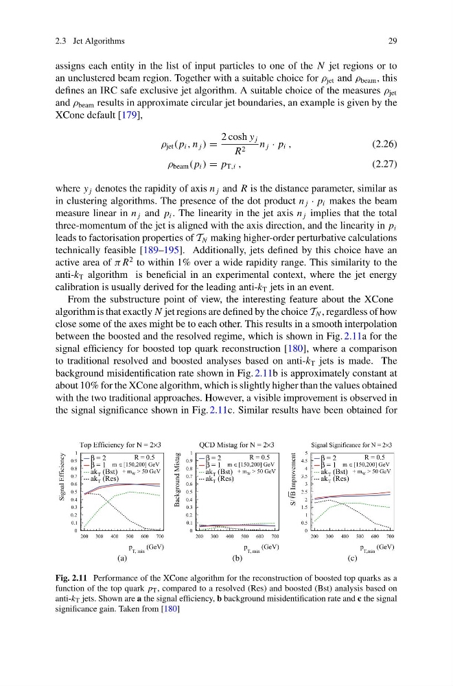
From the substructure point of view, the interesting feature about the XCone
algorithm is that exactly N jet regions are defined by the choice T N , regardless of how
close some of the axes might be to each other. This results in a smooth interpolation
between the boosted and the resolved regime, which is shown in Fig. 2.11a for the
signal efficiency for boosted top quark reconstruction [180], where a comparison
to traditional resolved and boosted analyses based on anti-k T jets is made. The
background misidentification rate shown in Fig. 2.11b is approximately constant at
about 10% for the XCone algorithm, which is slightly higher than the values obtained
with the two traditional approaches. However, a visible improvement is observed in
the signal significance shown in Fig. 2.11c. Similar results have been obtained for
(GeV)
T, min
p
200 300
400 500 600
700
Signal Efficiency
0
0.1
0.2
0.3
0.4
0.5
0.6
0.7
0.8
0.9
1
= 2
β
= 1
β
(Bst)
T
ak
(Res)
T
ak
R = 0.5
[150,200] GeV
∈
m
> 50 GeV
W
+ m
3
×
Top Efficiency for N = 2
(a)
(GeV)
T, min
p
200 300
400 500 600
700
Background Mistag
0
0.1
0.2
0.3
0.4
0.5
0.6
0.7
0.8
0.9
1
= 2
β
= 1
β
(Bst)
T
ak
(Res)
T
ak
R = 0.5
[150,200] GeV
∈
m
> 50 GeV
W
+ m
3
×
QCD Mistag for N = 2
(b)
(GeV)
T,min
p
200 300
400 500 600
700
Improvement
B
S/
0
0.5
1
1.5
2
2.5
3
3.5
4
4.5
5
= 2
β
= 1
β
(Bst)
T
ak
(Res)
T
ak
R = 0.5
[150,200] GeV
∈
m
> 50 GeV
W
+ m
3
×
Signal Significance for N = 2
(c)
Fig. 2.11 Performance of the XCone algorithm for the reconstruction of boosted top quarks as a
function of the top quark p T , compared to a resolved (Res) and boosted (Bst) analysis based on
anti-k T jets. Shown are a the signal efficiency, b background misidentification rate and c the signal
significance gain. Taken from [180]
29
assigns each entity in the list of input particles to one of the N jet regions or to
an unclustered beam region. Together with a suitable choice for ρ jet and ρ beam , this
defines an IRC safe exclusive jet algorithm. A suitable choice of the measures ρ jet
and ρ beam results in approximate circular jet boundaries, an example is given by the
XCone default [179],
ρ jet ( p i , n j ) =
2 cosh y j
R 2 n j · p i ,
(2.26)
ρ beam ( p i ) = p T,i ,
(2.27)
where y j denotes the rapidity of axis n j and R is the distance parameter, similar as
in clustering algorithms. The presence of the dot product n j · p i makes the beam
measure linear in n j and p i . The linearity in the jet axis n j implies that the total
three-momentum of the jet is aligned with the axis direction, and the linearity in p i
leads to factorisation properties of T N making higher-order perturbative calculations
technically feasible [189–195]. Additionally, jets defined by this choice have an
active area of π R
2 to within 1% over a wide rapidity range. This similarity to the
anti-k T algorithm is beneficial in an experimental context, where the jet energy
calibration is usually derived for the leading anti-k T jets in an event.
From the substructure point of view, the interesting feature about the XCone
algorithm is that exactly N jet regions are defined by the choice T N , regardless of how
close some of the axes might be to each other. This results in a smooth interpolation
between the boosted and the resolved regime, which is shown in Fig. 2.11a for the
signal efficiency for boosted top quark reconstruction [180], where a comparison
to traditional resolved and boosted analyses based on anti-k T jets is made. The
background misidentification rate shown in Fig. 2.11b is approximately constant at
about 10% for the XCone algorithm, which is slightly higher than the values obtained
with the two traditional approaches. However, a visible improvement is observed in
the signal significance shown in Fig. 2.11c. Similar results have been obtained for
(GeV)
T, min
p
200 300
400 500 600
700
Signal Efficiency
0
0.1
0.2
0.3
0.4
0.5
0.6
0.7
0.8
0.9
1
= 2
β
= 1
β
(Bst)
T
ak
(Res)
T
ak
R = 0.5
[150,200] GeV
∈
m
> 50 GeV
W
+ m
3
×
Top Efficiency for N = 2
(a)
(GeV)
T, min
p
200 300
400 500 600
700
Background Mistag
0
0.1
0.2
0.3
0.4
0.5
0.6
0.7
0.8
0.9
1
= 2
β
= 1
β
(Bst)
T
ak
(Res)
T
ak
R = 0.5
[150,200] GeV
∈
m
> 50 GeV
W
+ m
3
×
QCD Mistag for N = 2
(b)
(GeV)
T,min
p
200 300
400 500 600
700
Improvement
B
S/
0
0.5
1
1.5
2
2.5
3
3.5
4
4.5
5
= 2
β
= 1
β
(Bst)
T
ak
(Res)
T
ak
R = 0.5
[150,200] GeV
∈
m
> 50 GeV
W
+ m
3
×
Signal Significance for N = 2
(c)
Fig. 2.11 Performance of the XCone algorithm for the reconstruction of boosted top quarks as a
function of the top quark p T , compared to a resolved (Res) and boosted (Bst) analysis based on
anti-k T jets. Shown are a the signal efficiency, b background misidentification rate and c the signal
significance gain. Taken from [180]