

5.2 Various Sampling Methods
89
This is a probability distribution, so note the relation
i P i = 1.
The weather at a certain location changes daily, as s 1 → s 2 → s 1 → s 1 → · · · .
Consider a simple model to predict tomorrow’s weather. For example, if we make
the assumption that the day after a sunny day will be more sunny and the day after
a rainy day will be more rainy, this is a model called a Gothenburg weather model.
This is a Markov chain, as described below.
Markov chains are defined by transitions between states. However, we consider
only those whose state transitions are only dependent on the current state and not
on the past history. The above weather model is a Markov chain, assuming that the
next day’s weather depends only on the previous day’s weather.
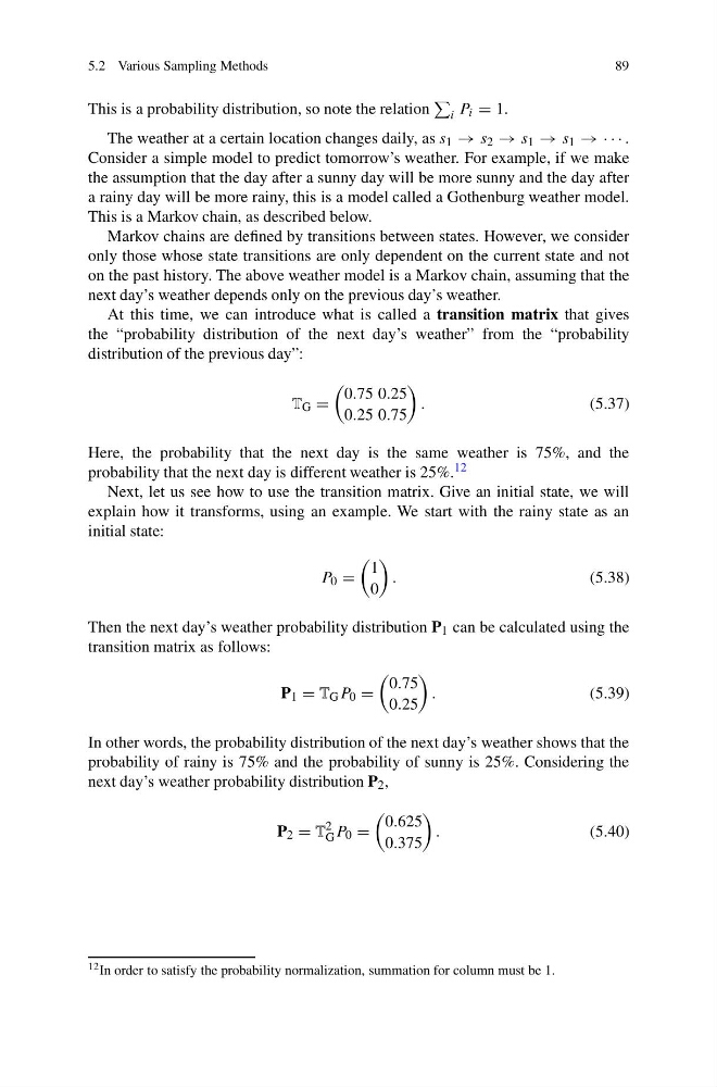
At this time, we can introduce what is called a transition matrix that gives
the “probability distribution of the next day’s weather” from the “probability
distribution of the previous day”:
T G =
0.75 0.25
0.25 0.75
.
(5.37)
Here, the probability that the next day is the same weather is 75%, and the
probability that the next day is different weather is 25%. 12
Next, let us see how to use the transition matrix. Give an initial state, we will
explain how it transforms, using an example. We start with the rainy state as an
initial state:
P 0 =
1
0
.
(5.38)
Then the next day’s weather probability distribution P 1 can be calculated using the
transition matrix as follows:
P 1 = T G P 0 =
0.75
0.25
.
(5.39)
In other words, the probability distribution of the next day’s weather shows that the
probability of rainy is 75% and the probability of sunny is 25%. Considering the
next day’s weather probability distribution P 2 ,
P 2 = T
2
G P 0 =
0.625
0.375
.
(5.40)
12 In order to satisfy the probability normalization, summation for column must be 1.
89
This is a probability distribution, so note the relation
i P i = 1.
The weather at a certain location changes daily, as s 1 → s 2 → s 1 → s 1 → · · · .
Consider a simple model to predict tomorrow’s weather. For example, if we make
the assumption that the day after a sunny day will be more sunny and the day after
a rainy day will be more rainy, this is a model called a Gothenburg weather model.
This is a Markov chain, as described below.
Markov chains are defined by transitions between states. However, we consider
only those whose state transitions are only dependent on the current state and not
on the past history. The above weather model is a Markov chain, assuming that the
next day’s weather depends only on the previous day’s weather.
At this time, we can introduce what is called a transition matrix that gives
the “probability distribution of the next day’s weather” from the “probability
distribution of the previous day”:
T G =
0.75 0.25
0.25 0.75
.
(5.37)
Here, the probability that the next day is the same weather is 75%, and the
probability that the next day is different weather is 25%. 12
Next, let us see how to use the transition matrix. Give an initial state, we will
explain how it transforms, using an example. We start with the rainy state as an
initial state:
P 0 =
1
0
.
(5.38)
Then the next day’s weather probability distribution P 1 can be calculated using the
transition matrix as follows:
P 1 = T G P 0 =
0.75
0.25
.
(5.39)
In other words, the probability distribution of the next day’s weather shows that the
probability of rainy is 75% and the probability of sunny is 25%. Considering the
next day’s weather probability distribution P 2 ,
P 2 = T
2
G P 0 =
0.625
0.375
.
(5.40)
12 In order to satisfy the probability normalization, summation for column must be 1.