

5.1 Central Limit Theorem and Its Role in Machine Learning
83
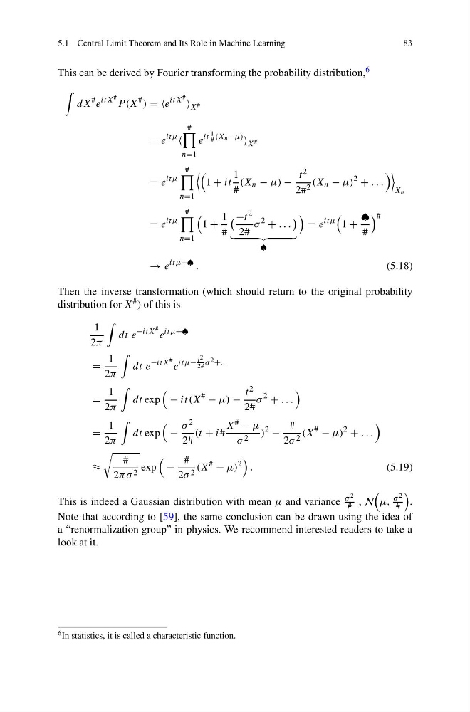
This can be derived by Fourier transforming the probability distribution, 6
dX
# e
itX #
P (X
# ) = =e
itX # X #
= e
itμ
#
n=1
e
it
1
# (X n −μ)
X #
= e
itμ
#
n=1
1 + it
1
#
(X n − μ) −
t 2
2# 2 (X n − μ)
2
+ . . .
X n
= e
itμ
#
n=1
1 +
1
#
−t 2
2#
σ
2
+ . . .
♠
= e
itμ
1 +
♠
#
#
→ e
itμ+♠ .
(5.18)
Then the inverse transformation (which should return to the original probability
distribution for X # ) of this is
1
2π
dt e
−itX #
e
itμ+♠
=
1
2π
dt e
−itX #
e
itμ−
t 2
2# σ 2 +...
=
1
2π
dt exp
− it (X
#
− μ) −
t 2
2#
σ
2
+ . . .
=
1
2π
dt exp
−
σ 2
2#
(t + i#
X # − μ
σ 2 )
2
−
#
2σ 2 (X
#
− μ)
2
+ . . .
≈
#
2πσ 2 exp
−
#
2σ 2 (X
#
− μ)
2
.
(5.19)
This is indeed a Gaussian distribution with mean μ and variance
σ 2
# , N
μ,
σ 2
#
.
Note that according to [59], the same conclusion can be drawn using the idea of
a “renormalization group” in physics. We recommend interested readers to take a
look at it.
6 In statistics, it is called a characteristic function.
83
This can be derived by Fourier transforming the probability distribution, 6
dX
# e
itX #
P (X
# ) = =e
itX # X #
= e
itμ
#
n=1
e
it
1
# (X n −μ)
X #
= e
itμ
#
n=1
1 + it
1
#
(X n − μ) −
t 2
2# 2 (X n − μ)
2
+ . . .
X n
= e
itμ
#
n=1
1 +
1
#
−t 2
2#
σ
2
+ . . .
♠
= e
itμ
1 +
♠
#
#
→ e
itμ+♠ .
(5.18)
Then the inverse transformation (which should return to the original probability
distribution for X # ) of this is
1
2π
dt e
−itX #
e
itμ+♠
=
1
2π
dt e
−itX #
e
itμ−
t 2
2# σ 2 +...
=
1
2π
dt exp
− it (X
#
− μ) −
t 2
2#
σ
2
+ . . .
=
1
2π
dt exp
−
σ 2
2#
(t + i#
X # − μ
σ 2 )
2
−
#
2σ 2 (X
#
− μ)
2
+ . . .
≈
#
2πσ 2 exp
−
#
2σ 2 (X
#
− μ)
2
.
(5.19)
This is indeed a Gaussian distribution with mean μ and variance
σ 2
# , N
μ,
σ 2
#
.
Note that according to [59], the same conclusion can be drawn using the idea of
a “renormalization group” in physics. We recommend interested readers to take a
look at it.
6 In statistics, it is called a characteristic function.