

82
5 Sampling
with
μ = =X, σ
2
= =(X − μ)
2
.
(5.15)
In other words, we can use a sampling average X # instead of the expectation value
μ = =X, if the number of samples # is enough large. So, to say it without worrying
about being misunderstood, there is no need to calculate the expectation value when
a large number of samples is possible. In fact, it is customary to calculate the
average value of observables by sampling instead of the exact expectation value
in the statistical mechanics of multi-degree-of-freedom systems in particle physics
and condensed matter physics. When the probability that X # converges to a certain
value μ at # → ∞ as in (5.14) is unity, we say that X # converges in probability to
μ.
Central limit theorem
Now let us bring back the customer in the previous example:
I know that (5.14) holds, but what’s the value of X
# after all?
Such an opinion would be natural in a sense. Equation (5.14) states that the sampling
average approaches the expectation value (that is a convergence in probability), but
does not tell how it approaches to the value. The central limit theorem actually tells
that to us:
P (X
# ) → N
μ,
σ 2
#
,
(5.16)
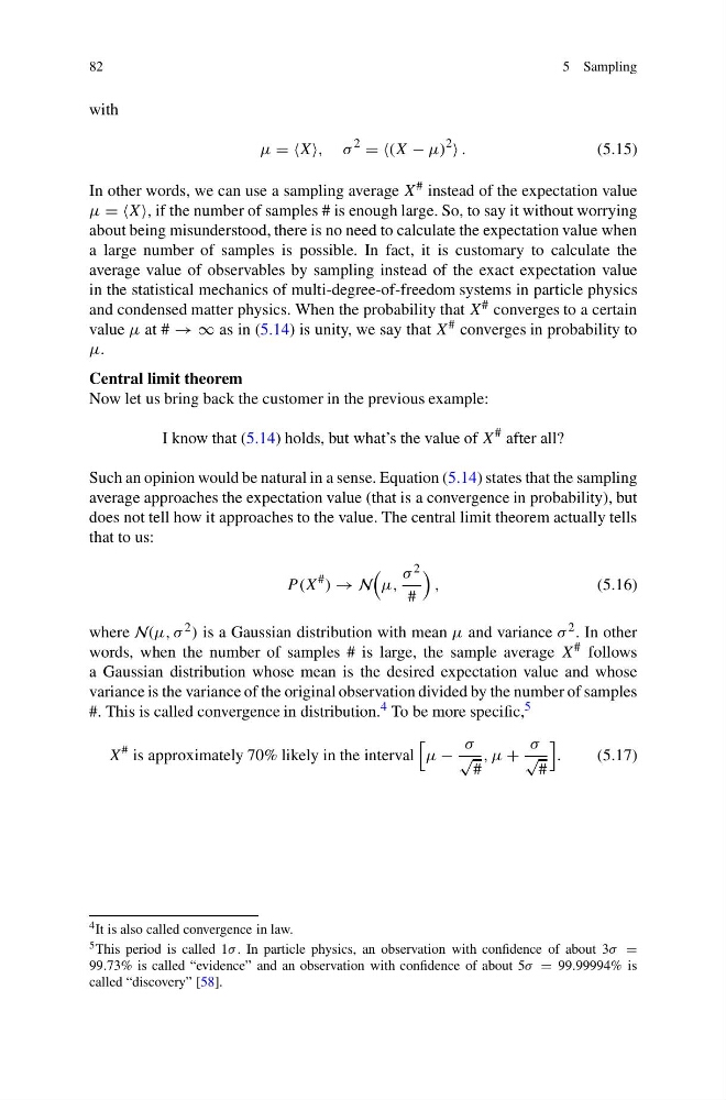
where N(μ, σ 2 ) is a Gaussian distribution with mean μ and variance σ 2 . In other
words, when the number of samples # is large, the sample average X # follows
a Gaussian distribution whose mean is the desired expectation value and whose
variance is the variance of the original observation divided by the number of samples
#. This is called convergence in distribution. 4 To be more specific, 5
X
# is approximately 70% likely in the interval
μ −
σ
√
#
, μ +
σ
√
#
.
(5.17)
4 It is also called convergence in law.
5 This period is called 1σ . In particle physics, an observation with confidence of about 3σ =
99.73% is called “evidence” and an observation with confidence of about 5σ = 99.99994% is
called “discovery” [58].
5 Sampling
with
μ = =X, σ
2
= =(X − μ)
2
.
(5.15)
In other words, we can use a sampling average X # instead of the expectation value
μ = =X, if the number of samples # is enough large. So, to say it without worrying
about being misunderstood, there is no need to calculate the expectation value when
a large number of samples is possible. In fact, it is customary to calculate the
average value of observables by sampling instead of the exact expectation value
in the statistical mechanics of multi-degree-of-freedom systems in particle physics
and condensed matter physics. When the probability that X # converges to a certain
value μ at # → ∞ as in (5.14) is unity, we say that X # converges in probability to
μ.
Central limit theorem
Now let us bring back the customer in the previous example:
I know that (5.14) holds, but what’s the value of X
# after all?
Such an opinion would be natural in a sense. Equation (5.14) states that the sampling
average approaches the expectation value (that is a convergence in probability), but
does not tell how it approaches to the value. The central limit theorem actually tells
that to us:
P (X
# ) → N
μ,
σ 2
#
,
(5.16)
where N(μ, σ 2 ) is a Gaussian distribution with mean μ and variance σ 2 . In other
words, when the number of samples # is large, the sample average X # follows
a Gaussian distribution whose mean is the desired expectation value and whose
variance is the variance of the original observation divided by the number of samples
#. This is called convergence in distribution. 4 To be more specific, 5
X
# is approximately 70% likely in the interval
μ −
σ
√
#
, μ +
σ
√
#
.
(5.17)
4 It is also called convergence in law.
5 This period is called 1σ . In particle physics, an observation with confidence of about 3σ =
99.73% is called “evidence” and an observation with confidence of about 5σ = 99.99994% is
called “discovery” [58].