

42
3 Basics of Neural Networks
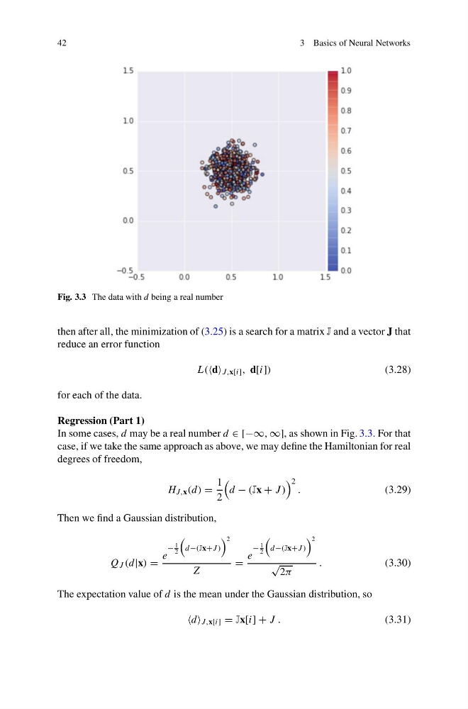
Fig. 3.3 The data with d being a real number
then after all, the minimization of (3.25) is a search for a matrix J and a vector J that
reduce an error function
L( J,x[i] , d[i])
(3.28)
for each of the data.
Regression (Part 1)
In some cases, d may be a real number d ∈ [−∞, ∞], as shown in Fig. 3.3. For that
case, if we take the same approach as above, we may define the Hamiltonian for real
degrees of freedom,
H J,x (d) =
1
2
d − (Jx + J )
2
.
(3.29)
Then we find a Gaussian distribution,
Q J (d|x) =
e
−
1
2
d−(Jx+J )
2
Z
=
e
−
1
2
d−(Jx+J )
2
√
2π
.
(3.30)
The expectation value of d is the mean under the Gaussian distribution, so
J,x[i] = Jx[i] + J .
(3.31)
3 Basics of Neural Networks
Fig. 3.3 The data with d being a real number
then after all, the minimization of (3.25) is a search for a matrix J and a vector J that
reduce an error function
L( J,x[i] , d[i])
(3.28)
for each of the data.
Regression (Part 1)
In some cases, d may be a real number d ∈ [−∞, ∞], as shown in Fig. 3.3. For that
case, if we take the same approach as above, we may define the Hamiltonian for real
degrees of freedom,
H J,x (d) =
1
2
d − (Jx + J )
2
.
(3.29)
Then we find a Gaussian distribution,
Q J (d|x) =
e
−
1
2
d−(Jx+J )
2
Z
=
e
−
1
2
d−(Jx+J )
2
√
2π
.
(3.30)
The expectation value of d is the mean under the Gaussian distribution, so
J,x[i] = Jx[i] + J .
(3.31)