

1.3 Machine Learning and Information Theory
7
Then, we should look for q i that makes this value as large as possible. In machine
learning, q i is varied to actually increase the amount equivalent to (1.14) as much
as possible. 5
By the way, if the number of data is large (# ≈ ∞), by the law of large numbers, 6
we have
# i
#
≈ p i ⇔ # i ≈ # · p i .
(1.17)
Here, # i must also be a large value, so according to Stirling’s formula (which is
familiar in physics), we find
# i ! ≈ #
# i
i .
(1.18)
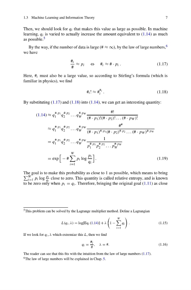
By substituting (1.17) and (1.18) into (1.14), we can get an interesting quantity:
(1.14) ≈ q
#·p 1
1
q
#·p 2
2
. . . q
#·p W
W
#!
(# · p 1 )!(# · p 2 )! . . . (# · p W )!
≈ q
#·p 1
1
q
#·p 2
2
. . . q
#·p W
W
# #
(# · p 1 ) #·p 1 (# · p 2 ) #·p 2 . . . (# · p W ) #·p W
= q
#·p 1
1
q
#·p 2
2
. . . q
#·p W
W
1
p
#·p 1
1 p
#·p 2
2
. . . p
#·p W
W
= exp
− #
W
i=1
p i log
p i
q i
.
(1.19)
The goal is to make this probability as close to 1 as possible, which means to bring
W
i=1 p i log
p i
q i
close to zero. This quantity is called relative entropy, and is known
to be zero only when p i = q i . Therefore, bringing the original goal (1.11) as close
5 This problem can be solved by the Lagrange multiplier method. Define a Lagrangian
L(q i , λ) = log[Eq. (1.14)] + λ
1 −
W
i=1
q i
.
(1.15)
If we look for q i , λ which extremize this L, then we find
q i =
# i
#
, λ = #.
(1.16)
The reader can see that this fits with the intuition from the law of large numbers (1.17).
6 The law of large numbers will be explained in Chap. 5.
7
Then, we should look for q i that makes this value as large as possible. In machine
learning, q i is varied to actually increase the amount equivalent to (1.14) as much
as possible. 5
By the way, if the number of data is large (# ≈ ∞), by the law of large numbers, 6
we have
# i
#
≈ p i ⇔ # i ≈ # · p i .
(1.17)
Here, # i must also be a large value, so according to Stirling’s formula (which is
familiar in physics), we find
# i ! ≈ #
# i
i .
(1.18)
By substituting (1.17) and (1.18) into (1.14), we can get an interesting quantity:
(1.14) ≈ q
#·p 1
1
q
#·p 2
2
. . . q
#·p W
W
#!
(# · p 1 )!(# · p 2 )! . . . (# · p W )!
≈ q
#·p 1
1
q
#·p 2
2
. . . q
#·p W
W
# #
(# · p 1 ) #·p 1 (# · p 2 ) #·p 2 . . . (# · p W ) #·p W
= q
#·p 1
1
q
#·p 2
2
. . . q
#·p W
W
1
p
#·p 1
1 p
#·p 2
2
. . . p
#·p W
W
= exp
− #
W
i=1
p i log
p i
q i
.
(1.19)
The goal is to make this probability as close to 1 as possible, which means to bring
W
i=1 p i log
p i
q i
close to zero. This quantity is called relative entropy, and is known
to be zero only when p i = q i . Therefore, bringing the original goal (1.11) as close
5 This problem can be solved by the Lagrange multiplier method. Define a Lagrangian
L(q i , λ) = log[Eq. (1.14)] + λ
1 −
W
i=1
q i
.
(1.15)
If we look for q i , λ which extremize this L, then we find
q i =
# i
#
, λ = #.
(1.16)
The reader can see that this fits with the intuition from the law of large numbers (1.17).
6 The law of large numbers will be explained in Chap. 5.