

12.3 Emergent Spacetime on Neural Networks
183
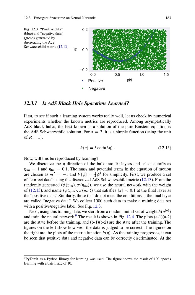
Fig. 12.3 “Positive data”
(blue) and “negative data”
(green) generated by
discretizing the AdS
Schwarzschild metric (12.13)
12.3.1 Is AdS Black Hole Spacetime Learned?
First, to see if such a learning system works really well, let us check by numerical
experiments whether the known metrics are reproduced. Among asymptotically
AdS black holes, the best known as a solution of the pure Einstein equation is
the AdS Schwarzschild solution. For d = 3, it is a simple function (using the unit
of R = 1),
h(η) = 3 coth(3η) .
(12.13)
Now, will this be reproduced by learning?
We discretize the η direction of the bulk into 10 layers and select cutoffs as
η ini = 1 and η fin = 0.1. The mass and potential terms in the equation of motion
are chosen as m 2 = −1 and V [φ] =
1
4 φ 4 for simplicity. First, we produce a set
of “correct data” using the discretized AdS Schwarzschild metric (12.13). From the
randomly generated (φ(η ini ), π(η ini )), we use the neural network with the weight
of (12.13), and name (φ(η ini ), π(η ini )) that satisfies |π| < 0.1 at the final layer as
the “positive data.” Similarly, those that do not meet the conditions at the final layer
are called “negative data.” We collect 1000 such data to make a training data set
with a positive/negative label. See Fig. 12.3.
Next, using this training data, we start from a random initial set of weight h(η (n) )
and train the neural network. 9 The result is shown in Fig. 12.4. The plots (a-1)(a-2)
are the state before the training, and (b-1)(b-2) are the state after the training. The
figures on the left show how well the data is judged to be correct. The figures on
the right are the plots of the metric function h(η). As the training progresses, it can
be seen that positive data and negative data can be correctly discriminated. At the
9 PyTorch as a Python library for learning was used. The figure shows the result of 100 epochs
learning with a batch size of 10.
183
Fig. 12.3 “Positive data”
(blue) and “negative data”
(green) generated by
discretizing the AdS
Schwarzschild metric (12.13)
12.3.1 Is AdS Black Hole Spacetime Learned?
First, to see if such a learning system works really well, let us check by numerical
experiments whether the known metrics are reproduced. Among asymptotically
AdS black holes, the best known as a solution of the pure Einstein equation is
the AdS Schwarzschild solution. For d = 3, it is a simple function (using the unit
of R = 1),
h(η) = 3 coth(3η) .
(12.13)
Now, will this be reproduced by learning?
We discretize the η direction of the bulk into 10 layers and select cutoffs as
η ini = 1 and η fin = 0.1. The mass and potential terms in the equation of motion
are chosen as m 2 = −1 and V [φ] =
1
4 φ 4 for simplicity. First, we produce a set
of “correct data” using the discretized AdS Schwarzschild metric (12.13). From the
randomly generated (φ(η ini ), π(η ini )), we use the neural network with the weight
of (12.13), and name (φ(η ini ), π(η ini )) that satisfies |π| < 0.1 at the final layer as
the “positive data.” Similarly, those that do not meet the conditions at the final layer
are called “negative data.” We collect 1000 such data to make a training data set
with a positive/negative label. See Fig. 12.3.
Next, using this training data, we start from a random initial set of weight h(η (n) )
and train the neural network. 9 The result is shown in Fig. 12.4. The plots (a-1)(a-2)
are the state before the training, and (b-1)(b-2) are the state after the training. The
figures on the left show how well the data is judged to be correct. The figures on
the right are the plots of the metric function h(η). As the training progresses, it can
be seen that positive data and negative data can be correctly discriminated. At the
9 PyTorch as a Python library for learning was used. The figure shows the result of 100 epochs
learning with a batch size of 10.