

152
9 Dynamical Systems and Neural Networks
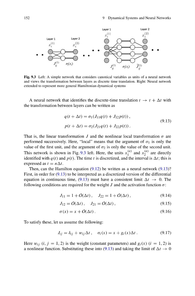
Fig. 9.3 Left: A simple network that considers canonical variables as units of a neural network
and views the transformation between layers as discrete time translation. Right: Neural network
extended to represent more general Hamiltonian dynamical systems
A neural network that identifies the discrete-time translation t → t + t with
the transformation between layers can be written as
q(t + = σ 1 (J 11 q(t) + J 12 p(t)) ,
p(t + = σ 2 (J 21 q(t) + J 22 p(t)) .
(9.13)
That is, the linear transformation J and the nonlinear local transformation σ are
performed successively. Here, “local” means that the argument of σ 1 is only the
value of the first unit, and the argument of σ 2 is only the value of the second unit.
This network is shown in Fig. 9.3 left. Here, the units x
(n)
1 and x
(n)
2 are directly
identified with q(t) and p(t). The time t is discretized, and the interval is t; this is
expressed as t = nnt.
Then, can the Hamilton equation (9.12) be written as a neural network (9.13)?
First, in order for (9.13) to be interpreted as a discretized version of the differential
equation in continuous time, (9.13) must have a consistent limit → 0. The
following conditions are required for the weight J and the activation function σ :
J 11 = 1 + O((t) , J 22 = 1 + O((t) ,
(9.14)
J 12 = O((t) , J 21 = O((t) ,
(9.15)
σ (x) = x + O((t) .
(9.16)
To satisfy these, let us assume the following:
J ij = δ ij + w ij , σ i (x) = x + g i (x))t .
(9.17)
Here w ij (i, j = 1, 2) is the weight (constant parameters) and g i (x) (i = 1, 2) is
a nonlinear function. Substituting these into (9.13) and taking the limit of → 0
9 Dynamical Systems and Neural Networks
Fig. 9.3 Left: A simple network that considers canonical variables as units of a neural network
and views the transformation between layers as discrete time translation. Right: Neural network
extended to represent more general Hamiltonian dynamical systems
A neural network that identifies the discrete-time translation t → t + t with
the transformation between layers can be written as
q(t + = σ 1 (J 11 q(t) + J 12 p(t)) ,
p(t + = σ 2 (J 21 q(t) + J 22 p(t)) .
(9.13)
That is, the linear transformation J and the nonlinear local transformation σ are
performed successively. Here, “local” means that the argument of σ 1 is only the
value of the first unit, and the argument of σ 2 is only the value of the second unit.
This network is shown in Fig. 9.3 left. Here, the units x
(n)
1 and x
(n)
2 are directly
identified with q(t) and p(t). The time t is discretized, and the interval is t; this is
expressed as t = nnt.
Then, can the Hamilton equation (9.12) be written as a neural network (9.13)?
First, in order for (9.13) to be interpreted as a discretized version of the differential
equation in continuous time, (9.13) must have a consistent limit → 0. The
following conditions are required for the weight J and the activation function σ :
J 11 = 1 + O((t) , J 22 = 1 + O((t) ,
(9.14)
J 12 = O((t) , J 21 = O((t) ,
(9.15)
σ (x) = x + O((t) .
(9.16)
To satisfy these, let us assume the following:
J ij = δ ij + w ij , σ i (x) = x + g i (x))t .
(9.17)
Here w ij (i, j = 1, 2) is the weight (constant parameters) and g i (x) (i = 1, 2) is
a nonlinear function. Substituting these into (9.13) and taking the limit of → 0