

9.2 Representation of Hamiltonian Dynamical System
151
In addition, there are neural networks created by imitating Hamilton equations 3
and also those that are made from second-order differential equations instead of the
first order. In this way, the skip connection that appeared to deepen and efficiently
train neural networks has a convenient form to interpret the neural network as a
discretized version of differential equations. 4
9.2 Representation of Hamiltonian Dynamical System
It is difficult to represent the time evolution of any Hamiltonian dynamical system
by a neural network. However, for a limited class of Hamiltonians, representation of
neural networks using local activation functions can be easily obtained. Let us look
at this. 5
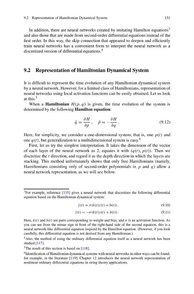
When a Hamiltonian H (p, q) is given, the time evolution of the system is
determined by the following Hamilton equation:
˙
q =
∂H
∂p
, ˙
p = −
∂H
∂q
.
(9.12)
Here, for simplicity, we consider a one-dimensional system, that is, one p(t) and
one q(t), but generalization to a multidimensional system is easy. 6
First, let us try the simplest interpretation. It takes the dimension of the vector
of each layer of the neural network as 2, equates it with (q(t), p(t)). Then we
discretize the t direction, and regard it as the depth direction in which the layers are
stacking. This method unfortunately shows that only free Hamiltonians (namely,
Hamiltonians consisting only of second-order polynomials in p and q) allow a
neural network representation, as we will see below.
3 For example, reference [115] gives a neural network that discretizes the following differential
equation based on the Hamiltonian dynamical system:
˙
y(t) = σ (k(t)z(t) + b(t)) ,
(9.10)
˙
z(t) = −σ (k(t)y(t) + b(t)) .
(9.11)
Here, k(t) and b(t) are parts corresponding to weight and bias, and σ is an activation function. As
you can see from the minus sign in front of the right-hand side of the second equation, this is a
neural network-like differential equation inspired by the Hamilton equation. (However, if you look
carefully, this differential equation is not derived from any Hamiltonian.)
4 Also, the method of using the ordinary differential equation itself as a neural network has been
studied [117].
5 The result of this section is based on [118].
6 Identification of Hamiltonian dynamical systems with neural networks in other ways can be found,
for example, in the literature [119]. Chapter 12 introduces the neural network representation of
nonlinear ordinary differential equations in string theory applications.
151
In addition, there are neural networks created by imitating Hamilton equations 3
and also those that are made from second-order differential equations instead of the
first order. In this way, the skip connection that appeared to deepen and efficiently
train neural networks has a convenient form to interpret the neural network as a
discretized version of differential equations. 4
9.2 Representation of Hamiltonian Dynamical System
It is difficult to represent the time evolution of any Hamiltonian dynamical system
by a neural network. However, for a limited class of Hamiltonians, representation of
neural networks using local activation functions can be easily obtained. Let us look
at this. 5
When a Hamiltonian H (p, q) is given, the time evolution of the system is
determined by the following Hamilton equation:
˙
q =
∂H
∂p
, ˙
p = −
∂H
∂q
.
(9.12)
Here, for simplicity, we consider a one-dimensional system, that is, one p(t) and
one q(t), but generalization to a multidimensional system is easy. 6
First, let us try the simplest interpretation. It takes the dimension of the vector
of each layer of the neural network as 2, equates it with (q(t), p(t)). Then we
discretize the t direction, and regard it as the depth direction in which the layers are
stacking. This method unfortunately shows that only free Hamiltonians (namely,
Hamiltonians consisting only of second-order polynomials in p and q) allow a
neural network representation, as we will see below.
3 For example, reference [115] gives a neural network that discretizes the following differential
equation based on the Hamiltonian dynamical system:
˙
y(t) = σ (k(t)z(t) + b(t)) ,
(9.10)
˙
z(t) = −σ (k(t)y(t) + b(t)) .
(9.11)
Here, k(t) and b(t) are parts corresponding to weight and bias, and σ is an activation function. As
you can see from the minus sign in front of the right-hand side of the second equation, this is a
neural network-like differential equation inspired by the Hamilton equation. (However, if you look
carefully, this differential equation is not derived from any Hamiltonian.)
4 Also, the method of using the ordinary differential equation itself as a neural network has been
studied [117].
5 The result of this section is based on [118].
6 Identification of Hamiltonian dynamical systems with neural networks in other ways can be found,
for example, in the literature [119]. Chapter 12 introduces the neural network representation of
nonlinear ordinary differential equations in string theory applications.