

9.1 Differential Equations and Neural Networks
149
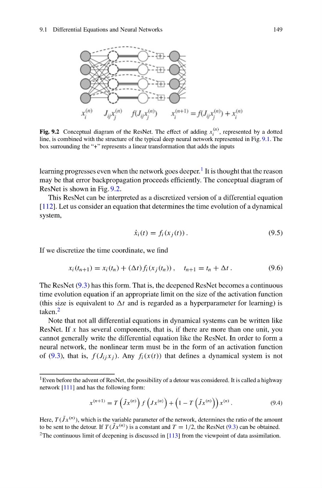
Fig. 9.2 Conceptual diagram of the ResNet. The effect of adding x
(n)
i , represented by a dotted
line, is combined with the structure of the typical deep neural network represented in Fig. 9.1. The
box surrounding the “+” represents a linear transformation that adds the inputs
learning progresses even when the network goes deeper. 1 It is thought that the reason
may be that error backpropagation proceeds efficiently. The conceptual diagram of
ResNet is shown in Fig. 9.2.
This ResNet can be interpreted as a discretized version of a differential equation
[112]. Let us consider an equation that determines the time evolution of a dynamical
system,
˙
x i (t) = f i (x j (t)) .
(9.5)
If we discretize the time coordinate, we find
x i (t n+1 ) = x i (t n ) + ((t)f i (x j (t n )) , t n+1 = t n + t .
(9.6)
The ResNet (9.3) has this form. That is, the deepened ResNet becomes a continuous
time evolution equation if an appropriate limit on the size of the activation function
(this size is equivalent to t and is regarded as a hyperparameter for learning) is
taken. 2
Note that not all differential equations in dynamical systems can be written like
ResNet. If x has several components, that is, if there are more than one unit, you
cannot generally write the differential equation like the ResNet. In order to form a
neural network, the nonlinear term must be in the form of an activation function
of (9.3), that is, f (J ij x j ). Any f i (x(t)) that defines a dynamical system is not
1 Even before the advent of ResNet, the possibility of a detour was considered. It is called a highway
network [111] and has the following form:
x
(n+1) = T
˜
J x
(n)
f
J x
(n)
+
1 − T
˜
J x
(n)
x
(n) .
(9.4)
Here, T ( ˜
J x (n) ), which is the variable parameter of the network, determines the ratio of the amount
to be sent to the detour. If T ( ˜
J x (n) ) is a constant and T = 1/2, the ResNet (9.3) can be obtained.
2 The continuous limit of deepening is discussed in [113] from the viewpoint of data assimilation.
149
Fig. 9.2 Conceptual diagram of the ResNet. The effect of adding x
(n)
i , represented by a dotted
line, is combined with the structure of the typical deep neural network represented in Fig. 9.1. The
box surrounding the “+” represents a linear transformation that adds the inputs
learning progresses even when the network goes deeper. 1 It is thought that the reason
may be that error backpropagation proceeds efficiently. The conceptual diagram of
ResNet is shown in Fig. 9.2.
This ResNet can be interpreted as a discretized version of a differential equation
[112]. Let us consider an equation that determines the time evolution of a dynamical
system,
˙
x i (t) = f i (x j (t)) .
(9.5)
If we discretize the time coordinate, we find
x i (t n+1 ) = x i (t n ) + ((t)f i (x j (t n )) , t n+1 = t n + t .
(9.6)
The ResNet (9.3) has this form. That is, the deepened ResNet becomes a continuous
time evolution equation if an appropriate limit on the size of the activation function
(this size is equivalent to t and is regarded as a hyperparameter for learning) is
taken. 2
Note that not all differential equations in dynamical systems can be written like
ResNet. If x has several components, that is, if there are more than one unit, you
cannot generally write the differential equation like the ResNet. In order to form a
neural network, the nonlinear term must be in the form of an activation function
of (9.3), that is, f (J ij x j ). Any f i (x(t)) that defines a dynamical system is not
1 Even before the advent of ResNet, the possibility of a detour was considered. It is called a highway
network [111] and has the following form:
x
(n+1) = T
˜
J x
(n)
f
J x
(n)
+
1 − T
˜
J x
(n)
x
(n) .
(9.4)
Here, T ( ˜
J x (n) ), which is the variable parameter of the network, determines the ratio of the amount
to be sent to the detour. If T ( ˜
J x (n) ) is a constant and T = 1/2, the ResNet (9.3) can be obtained.
2 The continuous limit of deepening is discussed in [113] from the viewpoint of data assimilation.