

148
9 Dynamical Systems and Neural Networks
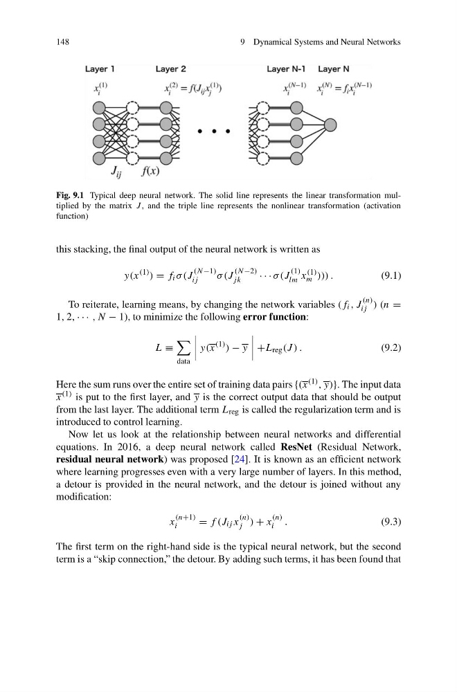
Fig. 9.1 Typical deep neural network. The solid line represents the linear transformation multiplied by the matrix J , and the triple line represents the nonlinear transformation (activation
function)
this stacking, the final output of the neural network is written as
y(x
(1) ) = f i σ (J
(N−1)
ij
σ (J
(N−2)
jk
· · · σ (J
(1)
lm x
(1)
m ))) .
(9.1)
To reiterate, learning means, by changing the network variables (f i , J
(n)
ij ) (n =
1, 2, · · · , N − 1), to minimize the following error function:
L ≡
data
y(x
(1) ) − y
+L reg (J ) .
(9.2)
Here the sum runs over the entire set of training data pairs {(x
(1) , y)}. The input data
x
(1) is put to the first layer, and y is the correct output data that should be output
from the last layer. The additional term L reg is called the regularization term and is
introduced to control learning.
Now let us look at the relationship between neural networks and differential
equations. In 2016, a deep neural network called ResNet (Residual Network,
residual neural network) was proposed [24]. It is known as an efficient network
where learning progresses even with a very large number of layers. In this method,
a detour is provided in the neural network, and the detour is joined without any
modification:
x
(n+1)
i
= f (J ij x
(n)
j ) + x
(n)
i .
(9.3)
The first term on the right-hand side is the typical neural network, but the second
term is a “skip connection,” the detour. By adding such terms, it has been found that
9 Dynamical Systems and Neural Networks
Fig. 9.1 Typical deep neural network. The solid line represents the linear transformation multiplied by the matrix J , and the triple line represents the nonlinear transformation (activation
function)
this stacking, the final output of the neural network is written as
y(x
(1) ) = f i σ (J
(N−1)
ij
σ (J
(N−2)
jk
· · · σ (J
(1)
lm x
(1)
m ))) .
(9.1)
To reiterate, learning means, by changing the network variables (f i , J
(n)
ij ) (n =
1, 2, · · · , N − 1), to minimize the following error function:
L ≡
data
y(x
(1) ) − y
+L reg (J ) .
(9.2)
Here the sum runs over the entire set of training data pairs {(x
(1) , y)}. The input data
x
(1) is put to the first layer, and y is the correct output data that should be output
from the last layer. The additional term L reg is called the regularization term and is
introduced to control learning.
Now let us look at the relationship between neural networks and differential
equations. In 2016, a deep neural network called ResNet (Residual Network,
residual neural network) was proposed [24]. It is known as an efficient network
where learning progresses even with a very large number of layers. In this method,
a detour is provided in the neural network, and the detour is joined without any
modification:
x
(n+1)
i
= f (J ij x
(n)
j ) + x
(n)
i .
(9.3)
The first term on the right-hand side is the typical neural network, but the second
term is a “skip connection,” the detour. By adding such terms, it has been found that