

134
7 Inverse Problems in Physics
term may be added:
≡ α
m−1
k=1
(x k − x k+1 )
2 .
(7.6)
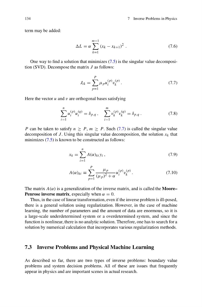
One way to find a solution that minimizes (7.5) is the singular value decomposition (SVD). Decompose the matrix J as follows:
J ik =
P
p=1
μ p u
(p)
i v
(p)
k .
(7.7)
Here the vector u and v are orthogonal bases satisfying
n
i=1
u
(p)
i u
(q)
i = δ p,q ,
m
i=1
v
(p)
k v
(q)
k = δ p,q .
(7.8)
P can be taken to satisfy n ≥ P , m ≥ P . Such (7.7) is called the singular value
decomposition of J . Using this singular value decomposition, the solution x k that
minimizes (7.5) is known to be constructed as follows:
x k =
n
i=1
A(α) ki y i ,
(7.9)
A(α) ki ≡
P
p=1
μ p
(μ p ) 2 + α
u
(p)
i v
(p)
k .
(7.10)
The matrix A(α) is a generalization of the inverse matrix, and is called the Moore–
Penrose inverse matrix, especially when α = 0.
Thus, in the case of linear transformation, even if the inverse problem is ill-posed,
there is a general solution using regularization. However, in the case of machine
learning, the number of parameters and the amount of data are enormous, so it is
a large-scale underdetermined system or a overdetermined system, and since the
function is nonlinear, there is no analytic solution. Therefore, one has to search for a
solution by numerical calculation that incorporates various regularization methods.
7.3 Inverse Problems and Physical Machine Learning
As described so far, there are two types of inverse problems: boundary value
problems and system decision problems. All of these are issues that frequently
appear in physics and are important scenes in actual research.
7 Inverse Problems in Physics
term may be added:
≡ α
m−1
k=1
(x k − x k+1 )
2 .
(7.6)
One way to find a solution that minimizes (7.5) is the singular value decomposition (SVD). Decompose the matrix J as follows:
J ik =
P
p=1
μ p u
(p)
i v
(p)
k .
(7.7)
Here the vector u and v are orthogonal bases satisfying
n
i=1
u
(p)
i u
(q)
i = δ p,q ,
m
i=1
v
(p)
k v
(q)
k = δ p,q .
(7.8)
P can be taken to satisfy n ≥ P , m ≥ P . Such (7.7) is called the singular value
decomposition of J . Using this singular value decomposition, the solution x k that
minimizes (7.5) is known to be constructed as follows:
x k =
n
i=1
A(α) ki y i ,
(7.9)
A(α) ki ≡
P
p=1
μ p
(μ p ) 2 + α
u
(p)
i v
(p)
k .
(7.10)
The matrix A(α) is a generalization of the inverse matrix, and is called the Moore–
Penrose inverse matrix, especially when α = 0.
Thus, in the case of linear transformation, even if the inverse problem is ill-posed,
there is a general solution using regularization. However, in the case of machine
learning, the number of parameters and the amount of data are enormous, so it is
a large-scale underdetermined system or a overdetermined system, and since the
function is nonlinear, there is no analytic solution. Therefore, one has to search for a
solution by numerical calculation that incorporates various regularization methods.
7.3 Inverse Problems and Physical Machine Learning
As described so far, there are two types of inverse problems: boundary value
problems and system decision problems. All of these are issues that frequently
appear in physics and are important scenes in actual research.