

7.2 Regularization in Inverse Problems
133
In many cases, although the forward problem satisfies the well-posedness, the
inverse problem is ill-posed. A typical example is the process of the many-body
system evolving to a macroscopic equilibrium. In a normal physical system in which
relaxation to an equilibrium state occurs, such as a thermal diffusion system, in order
to obtain the initial state before time evolution from the state after time evolution, a
very small fluctuation of the output value (from a perfect equilibrium state) must be
measured. In other words, relaxed systems generally do not have the stability (3).
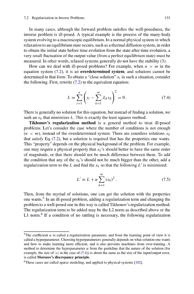
How can we deal with ill-posed problems? For example, when n > m in the
equation system (7.2), it is an overdetermined system, and solutions cannot be
determined in that form. To obtain a “close solution” x i in such a situation, consider
the following. First, rewrite (7.2) to the equivalent equation:
L ≡
n
i=1
y i −
m
k=1
J ik x k
2
= 0 .
(7.4)
There is generally no solution for this equation, but instead of finding a solution, we
seek an x k that minimizes L. This is exactly the least squares method.
Tikhonov’s regularization method is a general method to treat ill-posed
problems. Let’s consider the case where the number of conditions is not enough
(n < m), instead of the overdetermined system. There are countless solutions x k
that satisfy Eq. (7.2), but a solution is required that has the properties one wants.
This “property” depends on the physical background of the problem. For example,
one may require a physical property that x k ’s should better to have the same order
of magnitude, or that there should not be much difference between them. To add
the condition that any of the x k ’s should not be much bigger than the other, add a
regularization term to the L and find the x k so that the following L is minimized:
L
≡ L + α
m
k=1
(x k )
2 .
(7.5)
Then, from the myriad of solutions, one can get the solution with the properties
one wants. 5 In an ill-posed problem, adding a regularization term and changing the
problem to a well-posed one in this way is called Tikhonov’s regularization method.
The regularization term to be added may be the L2 norm as described above or the
L1 norm. 6 If a condition of no rattling is necessary, the following regularization
5 The coefficient α is called a regularization parameter, and from the learning point of view it is
called a hyperparameter. Choosing hyperparameters generally depends on what solution one wants
and how to make learning more efficient, and it also prevents machines from over-training. A
method to determine the hyperparameter α from the guideline that the nature of the solution (for
example, the size of |x| in the case of (7.4)) is about the same as the size of the input/output error,
is called Morozov’s discrepancy principle.
6 These cases are called sparse modeling, and applied to physical systems [102].
133
In many cases, although the forward problem satisfies the well-posedness, the
inverse problem is ill-posed. A typical example is the process of the many-body
system evolving to a macroscopic equilibrium. In a normal physical system in which
relaxation to an equilibrium state occurs, such as a thermal diffusion system, in order
to obtain the initial state before time evolution from the state after time evolution, a
very small fluctuation of the output value (from a perfect equilibrium state) must be
measured. In other words, relaxed systems generally do not have the stability (3).
How can we deal with ill-posed problems? For example, when n > m in the
equation system (7.2), it is an overdetermined system, and solutions cannot be
determined in that form. To obtain a “close solution” x i in such a situation, consider
the following. First, rewrite (7.2) to the equivalent equation:
L ≡
n
i=1
y i −
m
k=1
J ik x k
2
= 0 .
(7.4)
There is generally no solution for this equation, but instead of finding a solution, we
seek an x k that minimizes L. This is exactly the least squares method.
Tikhonov’s regularization method is a general method to treat ill-posed
problems. Let’s consider the case where the number of conditions is not enough
(n < m), instead of the overdetermined system. There are countless solutions x k
that satisfy Eq. (7.2), but a solution is required that has the properties one wants.
This “property” depends on the physical background of the problem. For example,
one may require a physical property that x k ’s should better to have the same order
of magnitude, or that there should not be much difference between them. To add
the condition that any of the x k ’s should not be much bigger than the other, add a
regularization term to the L and find the x k so that the following L is minimized:
L
≡ L + α
m
k=1
(x k )
2 .
(7.5)
Then, from the myriad of solutions, one can get the solution with the properties
one wants. 5 In an ill-posed problem, adding a regularization term and changing the
problem to a well-posed one in this way is called Tikhonov’s regularization method.
The regularization term to be added may be the L2 norm as described above or the
L1 norm. 6 If a condition of no rattling is necessary, the following regularization
5 The coefficient α is called a regularization parameter, and from the learning point of view it is
called a hyperparameter. Choosing hyperparameters generally depends on what solution one wants
and how to make learning more efficient, and it also prevents machines from over-training. A
method to determine the hyperparameter α from the guideline that the nature of the solution (for
example, the size of |x| in the case of (7.4)) is about the same as the size of the input/output error,
is called Morozov’s discrepancy principle.
6 These cases are called sparse modeling, and applied to physical systems [102].