

Column: Self-Learning Monte Carlo Method
125
The highest value of IS for ImageNet as of March 2019 is probably I S = 166.3
achieved in Ref. [99]. Interested readers should take a look at the image given in
the first page of the paper (which can be read for free). We are sure that the readers
will be surprised at how exquisite it is. For reference, if one uses Q J ∗ (d|x) which
processes a task classifying 1000 labels (classification using ImageNet), the full
mark for the score is I S = 1000 [93, 95].
Column: Self-Learning Monte Carlo Method
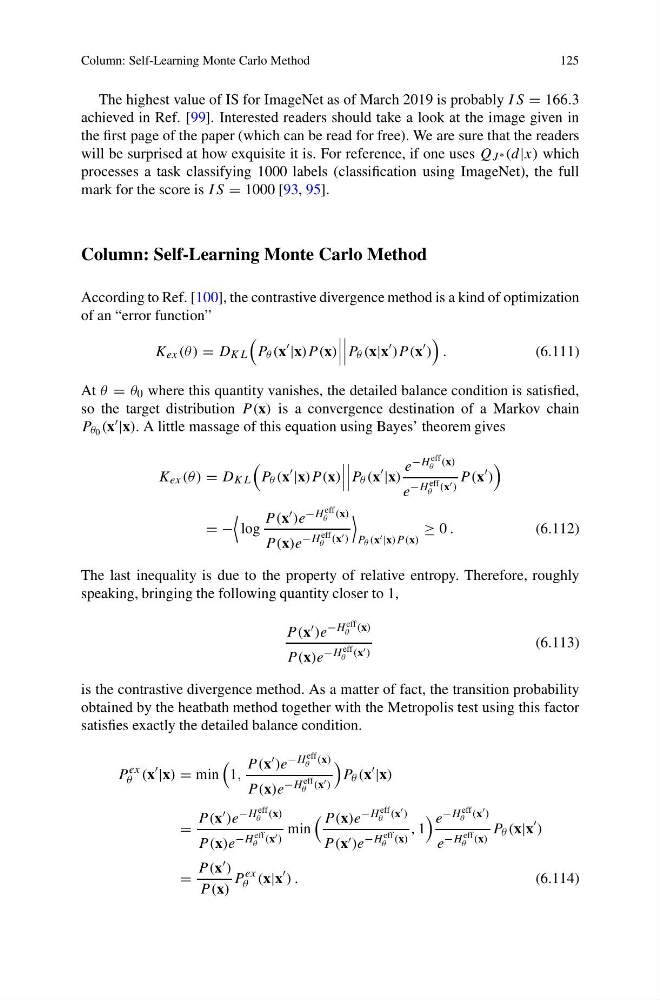
According to Ref. [100], the contrastive divergence method is a kind of optimization
of an “error function”
K ex (θ ) = D KL
P θ (x
|x)P (x)
Pθ (x|x
)P (x
)
.
(6.111)
At θ = θ 0 where this quantity vanishes, the detailed balance condition is satisfied,
so the target distribution P (x) is a convergence destination of a Markov chain
P θ 0 (x |x). A little massage of this equation using Bayes’ theorem gives
K ex (θ ) = D KL
P θ (x
|x)P (x)
Pθ (x
|x)
e −H eff
θ (x)
e
−H eff
θ (x )
P (x
)
= −
log
P (x )e −H eff
θ (x)
P (x)e
−H eff
θ (x )
P θ (x |x)P (x)
≥ 0 .
(6.112)
The last inequality is due to the property of relative entropy. Therefore, roughly
speaking, bringing the following quantity closer to 1,
P (x )e
−H eff
θ (x)
P (x)e −H eff
θ (x )
(6.113)
is the contrastive divergence method. As a matter of fact, the transition probability
obtained by the heatbath method together with the Metropolis test using this factor
satisfies exactly the detailed balance condition.
P
ex
θ (x
|x) = min
1,
P (x )e −H eff
θ (x)
P (x)e −H eff
θ (x )
P θ (x
|x)
=
P (x )e −H eff
θ (x)
P (x)e −H eff
θ (x )
min
P (x)e −H eff
θ (x )
P (x )e −H eff
θ (x)
, 1
e −H eff
θ (x )
e −H eff
θ (x)
P θ (x|x
)
=
P (x )
P (x)
P
ex
θ (x|x
) .
(6.114)
125
The highest value of IS for ImageNet as of March 2019 is probably I S = 166.3
achieved in Ref. [99]. Interested readers should take a look at the image given in
the first page of the paper (which can be read for free). We are sure that the readers
will be surprised at how exquisite it is. For reference, if one uses Q J ∗ (d|x) which
processes a task classifying 1000 labels (classification using ImageNet), the full
mark for the score is I S = 1000 [93, 95].
Column: Self-Learning Monte Carlo Method
According to Ref. [100], the contrastive divergence method is a kind of optimization
of an “error function”
K ex (θ ) = D KL
P θ (x
|x)P (x)
Pθ (x|x
)P (x
)
.
(6.111)
At θ = θ 0 where this quantity vanishes, the detailed balance condition is satisfied,
so the target distribution P (x) is a convergence destination of a Markov chain
P θ 0 (x |x). A little massage of this equation using Bayes’ theorem gives
K ex (θ ) = D KL
P θ (x
|x)P (x)
Pθ (x
|x)
e −H eff
θ (x)
e
−H eff
θ (x )
P (x
)
= −
log
P (x )e −H eff
θ (x)
P (x)e
−H eff
θ (x )
P θ (x |x)P (x)
≥ 0 .
(6.112)
The last inequality is due to the property of relative entropy. Therefore, roughly
speaking, bringing the following quantity closer to 1,
P (x )e
−H eff
θ (x)
P (x)e −H eff
θ (x )
(6.113)
is the contrastive divergence method. As a matter of fact, the transition probability
obtained by the heatbath method together with the Metropolis test using this factor
satisfies exactly the detailed balance condition.
P
ex
θ (x
|x) = min
1,
P (x )e −H eff
θ (x)
P (x)e −H eff
θ (x )
P θ (x
|x)
=
P (x )e −H eff
θ (x)
P (x)e −H eff
θ (x )
min
P (x)e −H eff
θ (x )
P (x )e −H eff
θ (x)
, 1
e −H eff
θ (x )
e −H eff
θ (x)
P θ (x|x
)
=
P (x )
P (x)
P
ex
θ (x|x
) .
(6.114)