

6.2 Boltzmann Machine
105
Here
P =
dx P (x) • (x)
(6.8)
represents the expectation value by the probability distribution P .
Training in actual cases
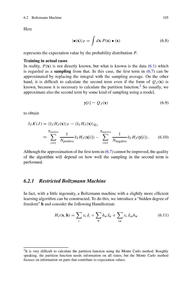
In reality, P (x) is not directly known, but what is known is the data (6.1) which
is regarded as a sampling from that. In this case, the first term in (6.7) can be
approximated by replacing the integral with the sampling average. On the other
hand, it is difficult to calculate the second term even if the form of Q J (x) is
known, because it is necessary to calculate the partition function. 2 So usually, we
approximate also the second term by some kind of sampling using a model,
y[i] ∼ Q J (x)
(6.9)
to obtain
∂ J K(J ) = =∂ J H J (x) P − −∂ J H J (x) Q J
≈
N positive
i=1
1
N positive
∂ J H J (x[i]) −
N negative
i=1
1
N negative
∂ J H J (y[i]) .
(6.10)
Although the approximation of the first term in (6.7) cannot be improved, the quality
of the algorithm will depend on how well the sampling in the second term is
performed.
6.2.1 Restricted Boltzmann Machine
In fact, with a little ingenuity, a Boltzmann machine with a slightly more efficient
learning algorithm can be constructed. To do this, we introduce a “hidden degree of
freedom” h and consider the following Hamiltonian:
H J (x, h) =
i
x i J i +
α
h α J α +
iα
x i J iα h α
(6.11)
2 It is very difficult to calculate the partition function using the Monte Carlo method. Roughly
speaking, the partition function needs information on all states, but the Monte Carlo method
focuses on information on parts that contribute to expectation values.
105
Here
P =
dx P (x) • (x)
(6.8)
represents the expectation value by the probability distribution P .
Training in actual cases
In reality, P (x) is not directly known, but what is known is the data (6.1) which
is regarded as a sampling from that. In this case, the first term in (6.7) can be
approximated by replacing the integral with the sampling average. On the other
hand, it is difficult to calculate the second term even if the form of Q J (x) is
known, because it is necessary to calculate the partition function. 2 So usually, we
approximate also the second term by some kind of sampling using a model,
y[i] ∼ Q J (x)
(6.9)
to obtain
∂ J K(J ) = =∂ J H J (x) P − −∂ J H J (x) Q J
≈
N positive
i=1
1
N positive
∂ J H J (x[i]) −
N negative
i=1
1
N negative
∂ J H J (y[i]) .
(6.10)
Although the approximation of the first term in (6.7) cannot be improved, the quality
of the algorithm will depend on how well the sampling in the second term is
performed.
6.2.1 Restricted Boltzmann Machine
In fact, with a little ingenuity, a Boltzmann machine with a slightly more efficient
learning algorithm can be constructed. To do this, we introduce a “hidden degree of
freedom” h and consider the following Hamiltonian:
H J (x, h) =
i
x i J i +
α
h α J α +
iα
x i J iα h α
(6.11)
2 It is very difficult to calculate the partition function using the Monte Carlo method. Roughly
speaking, the partition function needs information on all states, but the Monte Carlo method
focuses on information on parts that contribute to expectation values.