

104
6 Unsupervised Deep Learning
Even in this case, we assume that there exists some probability distribution P (x),
x[i] ∼ P (x) .
(6.2)
So now, let us consider that there is a model Q J (x), that is, a probability distribution
with a set of parameters J , and we want to make it closer to P (x). In other words,
we want to reduce
K(J ) =
dx P (x) log
P (x)
Q J (x)
.
(6.3)
Once this minimization is achieved, Q J (x) can be used to create “fake” data.
6.2 Boltzmann Machine
First, as usual, we consider a “statistical mechanics” model as Q J (x). For example,
consider a Hamiltonian with an interaction for each component of x as
H J (x) =
i
x i J i +
ij
x i J ij x j + . . .
(6.4)
and the model is given as
Q J (x) =
e −H J (x)
Z J
.
(6.5)
It is only necessary to adjust the “coupling constant” J to reduce (6.3). This is
called a Boltzmann machine. The simplest algorithm would be to differentiate (6.3)
and use the derivative to change the values of J :
J ← J − J K(J ).
(6.6)
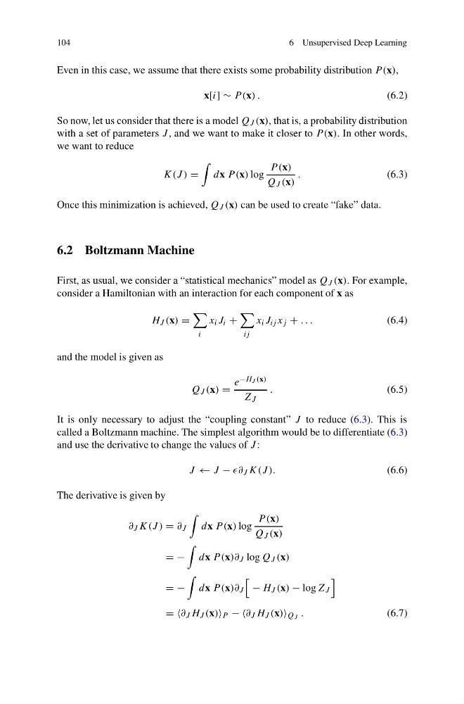
The derivative is given by
∂ J K(J ) = ∂ J
dx P (x) log
P (x)
Q J (x)
= −
dx P (x)∂ J log Q J (x)
= −
dx P (x)∂ J
− H J (x) − log Z J
= =∂ J H J (x) P − −∂ J H J (x) Q J .
(6.7)
6 Unsupervised Deep Learning
Even in this case, we assume that there exists some probability distribution P (x),
x[i] ∼ P (x) .
(6.2)
So now, let us consider that there is a model Q J (x), that is, a probability distribution
with a set of parameters J , and we want to make it closer to P (x). In other words,
we want to reduce
K(J ) =
dx P (x) log
P (x)
Q J (x)
.
(6.3)
Once this minimization is achieved, Q J (x) can be used to create “fake” data.
6.2 Boltzmann Machine
First, as usual, we consider a “statistical mechanics” model as Q J (x). For example,
consider a Hamiltonian with an interaction for each component of x as
H J (x) =
i
x i J i +
ij
x i J ij x j + . . .
(6.4)
and the model is given as
Q J (x) =
e −H J (x)
Z J
.
(6.5)
It is only necessary to adjust the “coupling constant” J to reduce (6.3). This is
called a Boltzmann machine. The simplest algorithm would be to differentiate (6.3)
and use the derivative to change the values of J :
J ← J − J K(J ).
(6.6)
The derivative is given by
∂ J K(J ) = ∂ J
dx P (x) log
P (x)
Q J (x)
= −
dx P (x)∂ J log Q J (x)
= −
dx P (x)∂ J
− H J (x) − log Z J
= =∂ J H J (x) P − −∂ J H J (x) Q J .
(6.7)