

38
Overall, the demand function in total is expressed as
D =
+
+
+
Food Feed Eth Ex
(5.13)
Finally, at the equilibrium, it holds that
D Q
=
(5.14)
5.3 Simulation
5.3.1 Overall design
We have to introduce some assumptions for our simulation analysis. Our simulation
begins 2007 and ends at 2020. The corn market in 2007 and 2008 was in an unusual
situation caused by unexpected factors such as the financial crisis. Since our model
is recursive, including these noises prevents us to analyze the mainstream trend in the
grain market. Thus we avoid 2009 as the initial year. In addition, this method allows
us to see how unusual the actual situation was in 2008 by comparing the actual value
with the equilibrium value which is solely determined by supply and demand.
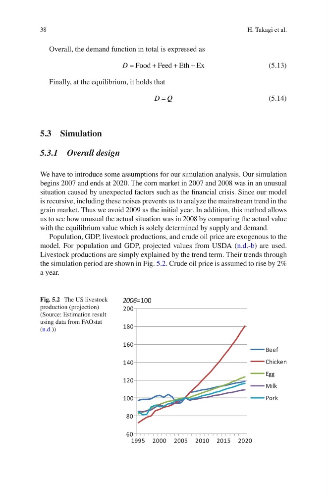
Population, GDP, livestock productions, and crude oil price are exogenous to the
model. For population and GDP, projected values from USDA (n.d.-b) are used.
Livestock productions are simply explained by the trend term. Their trends through
the simulation period are shown in Fig. 5.2. Crude oil price is assumed to rise by 2%
a year.
60
80
100
120
140
160
180
200
1995 2000 2005 2010 2015 2020
Beef
Chicken
Egg
Milk
Pork
2006=100
Fig. 5.2 The US livestock
production (projection)
(Source: Estimation result
using data from FAOstat
(n.d.))
H. Takagi et al.
Overall, the demand function in total is expressed as
D =
+
+
+
Food Feed Eth Ex
(5.13)
Finally, at the equilibrium, it holds that
D Q
=
(5.14)
5.3 Simulation
5.3.1 Overall design
We have to introduce some assumptions for our simulation analysis. Our simulation
begins 2007 and ends at 2020. The corn market in 2007 and 2008 was in an unusual
situation caused by unexpected factors such as the financial crisis. Since our model
is recursive, including these noises prevents us to analyze the mainstream trend in the
grain market. Thus we avoid 2009 as the initial year. In addition, this method allows
us to see how unusual the actual situation was in 2008 by comparing the actual value
with the equilibrium value which is solely determined by supply and demand.
Population, GDP, livestock productions, and crude oil price are exogenous to the
model. For population and GDP, projected values from USDA (n.d.-b) are used.
Livestock productions are simply explained by the trend term. Their trends through
the simulation period are shown in Fig. 5.2. Crude oil price is assumed to rise by 2%
a year.
60
80
100
120
140
160
180
200
1995 2000 2005 2010 2015 2020
Beef
Chicken
Egg
Milk
Pork
2006=100
Fig. 5.2 The US livestock
production (projection)
(Source: Estimation result
using data from FAOstat
(n.d.))
H. Takagi et al.