

34
regarded as one of the solutions. Expansion of demand for corn and its higher price
will contribute to their revenues and reduction of governmental expenditures. It is
misleading to judge for or against biofuel production with the fixed view that higher
price is always harmful.
For these reasons, cost-benefit analysis should be carried out. In this study, we
aim to find the most economically beneficial policies with regards to the US bioethanol production. The next section overviews the model structure of the US corn
market incorporating bioethanol. In the third section, we will show the simulation
results across five scenarios. In the fourth section, we will outline the method to
calculate the benefits and costs to each stakeholder. Our conclusion is presented in
the fifth section.
5.2 The Model Structure
5.2.1 Overview of the Model
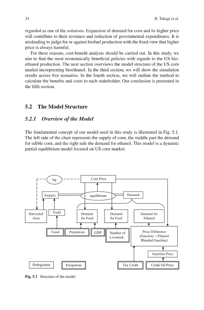
The fundamental concept of our model used in this study is illustrated in Fig. 5.1.
The left side of the chart represents the supply of corn, the middle part the demand
for edible corn, and the right side the demand for ethanol. This model is a dynamic
partial equilibrium model focused on US corn market.
Yield
Su pply
Harvested
Area
Corn Price
Gasoline Price
Price Difference
(GasolineJEthanol
Blended Gasoline)
Demand for
Ethanol
Demand
for Feed
Demand
Demand
for Food
equilibrium
Trend
Population
GDP
Number of
Livestock
Tax Credit
Crude Oil Price
Endogenous
Exogenous
lag
Fig. 5.1 Structure of the model
H. Takagi et al.
regarded as one of the solutions. Expansion of demand for corn and its higher price
will contribute to their revenues and reduction of governmental expenditures. It is
misleading to judge for or against biofuel production with the fixed view that higher
price is always harmful.
For these reasons, cost-benefit analysis should be carried out. In this study, we
aim to find the most economically beneficial policies with regards to the US bioethanol production. The next section overviews the model structure of the US corn
market incorporating bioethanol. In the third section, we will show the simulation
results across five scenarios. In the fourth section, we will outline the method to
calculate the benefits and costs to each stakeholder. Our conclusion is presented in
the fifth section.
5.2 The Model Structure
5.2.1 Overview of the Model
The fundamental concept of our model used in this study is illustrated in Fig. 5.1.
The left side of the chart represents the supply of corn, the middle part the demand
for edible corn, and the right side the demand for ethanol. This model is a dynamic
partial equilibrium model focused on US corn market.
Yield
Su pply
Harvested
Area
Corn Price
Gasoline Price
Price Difference
(GasolineJEthanol
Blended Gasoline)
Demand for
Ethanol
Demand
for Feed
Demand
Demand
for Food
equilibrium
Trend
Population
GDP
Number of
Livestock
Tax Credit
Crude Oil Price
Endogenous
Exogenous
lag
Fig. 5.1 Structure of the model
H. Takagi et al.