

74
3 Investigation of Euler–Bernoulli Beams in the Elastic Range
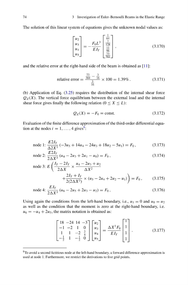
The solution of this linear system of equations gives the unknown nodal values as:
⎡
⎢
⎢
⎣
u 2
u 3
u 4
u 5
⎤
⎥
⎥
⎦ = −
F 0 L
3
E I Y
⎡
⎢
⎢
⎢
⎣
1
64
7
128
11
96
73
384
⎤
⎥
⎥
⎥
⎦
,
(3.170)
and the relative error at the right-hand side of the beam is obtained as [11]:
relative error =
73
384
−
3
16
3
16
× 100 = 1.39% .
(3.171)
(b) Application of Eq. (3.25) requires the distribution of the internal shear force
Q Z (X ). The vertical force equilibrium between the external load and the internal
shear force gives finally the following relation (0 ≤ X ≤ L):
Q Z (X ) = −F 0 = const.
(3.172)
Evaluation of the finite difference approximation of the third-order differential equation at the nodes i = 1, . . . , 4 gives
9 :
node 1:
E2I Y
2X 3 (−3u 5 + 14u 4 − 24u 3 + 18u 2 − 5u 1 ) = F 0 ,
(3.173)
node 2:
E2I Y
2X 3 (u 4 − 2u 3 + 2u 1 − u 0 ) = F 0 ,
(3.174)
node 3: E
I Y − 2I Y
2X
×
u 4 − 2u 3 + u 2
X 2
+
2I Y + I Y
2(2X 3 )
× (u 5 − 2u 4 + 2u 2 − u 1 )
= F 0 ,
(3.175)
node 4:
E I Y
2X 3 (u 6 − 2u 5 + 2u 3 − u 2 ) = F 0 ,
(3.176)
Using again the conditions from the left-hand boundary, i.e., u 1 = 0 and u 0 = u 2
as well as the condition that the moment is zero at the right-hand boundary, i.e.
u 6 = −u 4 + 2u 5 , the matrix notation is obtained as:
⎡
⎢
⎢
⎣
18 −24 14 −3
−1 −2 1 0
1 1 −2
3
4
−
1
2
1 −
1
2
0
⎤
⎥
⎥
⎦
⎡
⎢
⎢
⎣
u 2
u 3
u 4
u 5
⎤
⎥
⎥
⎦ =
X
3 F 0
E I Y
⎡
⎢
⎢
⎢
⎣
1
1
1
1
⎤
⎥
⎥
⎥
⎦
.
(3.177)
9 To avoid a second fictitious node at the left-hand boundary, a forward difference approximation is
used at node 1. Furthermore, we restrict the derivations to five grid points.
3 Investigation of Euler–Bernoulli Beams in the Elastic Range
The solution of this linear system of equations gives the unknown nodal values as:
⎡
⎢
⎢
⎣
u 2
u 3
u 4
u 5
⎤
⎥
⎥
⎦ = −
F 0 L
3
E I Y
⎡
⎢
⎢
⎢
⎣
1
64
7
128
11
96
73
384
⎤
⎥
⎥
⎥
⎦
,
(3.170)
and the relative error at the right-hand side of the beam is obtained as [11]:
relative error =
73
384
−
3
16
3
16
× 100 = 1.39% .
(3.171)
(b) Application of Eq. (3.25) requires the distribution of the internal shear force
Q Z (X ). The vertical force equilibrium between the external load and the internal
shear force gives finally the following relation (0 ≤ X ≤ L):
Q Z (X ) = −F 0 = const.
(3.172)
Evaluation of the finite difference approximation of the third-order differential equation at the nodes i = 1, . . . , 4 gives
9 :
node 1:
E2I Y
2X 3 (−3u 5 + 14u 4 − 24u 3 + 18u 2 − 5u 1 ) = F 0 ,
(3.173)
node 2:
E2I Y
2X 3 (u 4 − 2u 3 + 2u 1 − u 0 ) = F 0 ,
(3.174)
node 3: E
I Y − 2I Y
2X
×
u 4 − 2u 3 + u 2
X 2
+
2I Y + I Y
2(2X 3 )
× (u 5 − 2u 4 + 2u 2 − u 1 )
= F 0 ,
(3.175)
node 4:
E I Y
2X 3 (u 6 − 2u 5 + 2u 3 − u 2 ) = F 0 ,
(3.176)
Using again the conditions from the left-hand boundary, i.e., u 1 = 0 and u 0 = u 2
as well as the condition that the moment is zero at the right-hand boundary, i.e.
u 6 = −u 4 + 2u 5 , the matrix notation is obtained as:
⎡
⎢
⎢
⎣
18 −24 14 −3
−1 −2 1 0
1 1 −2
3
4
−
1
2
1 −
1
2
0
⎤
⎥
⎥
⎦
⎡
⎢
⎢
⎣
u 2
u 3
u 4
u 5
⎤
⎥
⎥
⎦ =
X
3 F 0
E I Y
⎡
⎢
⎢
⎢
⎣
1
1
1
1
⎤
⎥
⎥
⎥
⎦
.
(3.177)
9 To avoid a second fictitious node at the left-hand boundary, a forward difference approximation is
used at node 1. Furthermore, we restrict the derivations to five grid points.