

60
3 Investigation of Euler–Bernoulli Beams in the Elastic Range
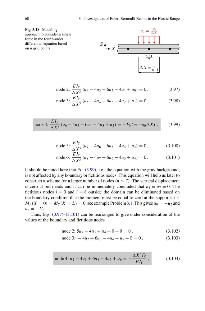
Fig. 3.18 Modeling
approach to consider a single
force in the fourth-order
differential equation based
on n grid points
node 2:
E I Y
X 3 (u 4 − 4u 3 + 6u 2 − 4u 1 + u 0 ) = 0 ,
(3.97)
node 3:
E I Y
X 3 (u 5 − 4u 4 + 6u 3 − 4u 2 + u 1 ) = 0 ,
(3.98)
node 4:
E I Y
X 3 (u 6 − 4u 5 + 6u 4 − 4u 3 + u 2 ) = −F 0 (= −q 0 ) ,
(3.99)
node 5:
E I Y
X 3 (u 7 − 4u 6 + 6u 5 − 4u 4 + u 3 ) = 0 ,
(3.100)
node 6:
E I Y
X 3 (u 8 − 4u 7 + 6u 6 − 4u 5 + u 4 ) = 0 .
(3.101)
It should be noted here that Eq. (3.99), i.e., the equation with the gray background,
is not affected by any boundary or fictitious nodes. This equation will help us later to
construct a scheme for a larger number of nodes (n > 7). The vertical displacement
is zero at both ends and it can be immediately concluded that u 1 = u 7 = 0. The
fictitious nodes i = 0 and i = 8 outside the domain can be eliminated based on
the boundary condition that the moment must be equal to zero at the supports, i.e.
M Y (X = 0) = M Y (X = L) = 0, see example Problem 3.1. This gives u 0 = −u 2 and
u 8 = −U 6 .
Thus, Eqs. (3.97)–(3.101) can be rearranged to give under consideration of the
values of the boundary and fictitious nodes
node 2: 5u 2 − 4u 3 + u 4 + 0 + 0 = 0 ,
(3.102)
node 3: − 4u 2 + 6u 3 − 4u 4 + u 5 + 0 = 0 ,
(3.103)
node 4: u 2 − 4u 3 + 6u 4 − 4u 5 + u 6 = −
3 F 0
E I Y
,
(3.104)
3 Investigation of Euler–Bernoulli Beams in the Elastic Range
Fig. 3.18 Modeling
approach to consider a single
force in the fourth-order
differential equation based
on n grid points
node 2:
E I Y
X 3 (u 4 − 4u 3 + 6u 2 − 4u 1 + u 0 ) = 0 ,
(3.97)
node 3:
E I Y
X 3 (u 5 − 4u 4 + 6u 3 − 4u 2 + u 1 ) = 0 ,
(3.98)
node 4:
E I Y
X 3 (u 6 − 4u 5 + 6u 4 − 4u 3 + u 2 ) = −F 0 (= −q 0 ) ,
(3.99)
node 5:
E I Y
X 3 (u 7 − 4u 6 + 6u 5 − 4u 4 + u 3 ) = 0 ,
(3.100)
node 6:
E I Y
X 3 (u 8 − 4u 7 + 6u 6 − 4u 5 + u 4 ) = 0 .
(3.101)
It should be noted here that Eq. (3.99), i.e., the equation with the gray background,
is not affected by any boundary or fictitious nodes. This equation will help us later to
construct a scheme for a larger number of nodes (n > 7). The vertical displacement
is zero at both ends and it can be immediately concluded that u 1 = u 7 = 0. The
fictitious nodes i = 0 and i = 8 outside the domain can be eliminated based on
the boundary condition that the moment must be equal to zero at the supports, i.e.
M Y (X = 0) = M Y (X = L) = 0, see example Problem 3.1. This gives u 0 = −u 2 and
u 8 = −U 6 .
Thus, Eqs. (3.97)–(3.101) can be rearranged to give under consideration of the
values of the boundary and fictitious nodes
node 2: 5u 2 − 4u 3 + u 4 + 0 + 0 = 0 ,
(3.102)
node 3: − 4u 2 + 6u 3 − 4u 4 + u 5 + 0 = 0 ,
(3.103)
node 4: u 2 − 4u 3 + 6u 4 − 4u 5 + u 6 = −
3 F 0
E I Y
,
(3.104)