

54
3 Investigation of Euler–Bernoulli Beams in the Elastic Range
u 6 = 2u 5 − u 4 ,
(3.74)
u 7 = 4u 5 − 4u 4 + u 3 +
q 0 X
4
E I Y
.
(3.75)
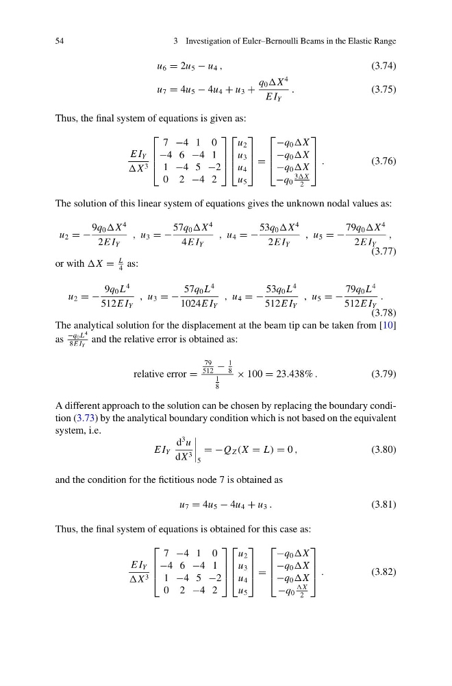
Thus, the final system of equations is given as:
E I Y
X 3
⎡
⎢
⎢
⎣
7 −4 1 0
−4 6 −4 1
1 −4 5 −2
0 2 −4 2
⎤
⎥
⎥
⎦
⎡
⎢
⎢
⎣
u 2
u 3
u 4
u 5
⎤
⎥
⎥
⎦ =
⎡
⎢
⎢
⎣
−q 0 X
−q 0 X
−q 0 X
−q 0
3X
2
⎤
⎥
⎥
⎦ .
(3.76)
The solution of this linear system of equations gives the unknown nodal values as:
u 2 = −
9q 0 X
4
2E I Y
, u 3 = −
57q 0 X
4
4E I Y
, u 4 = −
53q 0 X
4
2E I Y
, u 5 = −
79q 0 X
4
2E I Y
,
(3.77)
or with X =
L
4
as:
u 2 = −
9q 0 L
4
512E I Y
, u 3 = −
57q 0 L
4
1024E I Y
, u 4 = −
53q 0 L
4
512E I Y
, u 5 = −
79q 0 L
4
512E I Y
.
(3.78)
The analytical solution for the displacement at the beam tip can be taken from [10]
as
−q 0 L
4
8E I Y
and the relative error is obtained as:
relative error =
79
512
−
1
8
1
8
× 100 = 23.438% .
(3.79)
A different approach to the solution can be chosen by replacing the boundary condition (3.73) by the analytical boundary condition which is not based on the equivalent
system, i.e.
E I Y
d
3 u
dX 3
5
= −Q Z (X = L) = 0 ,
(3.80)
and the condition for the fictitious node 7 is obtained as
u 7 = 4u 5 − 4u 4 + u 3 .
(3.81)
Thus, the final system of equations is obtained for this case as:
E I Y
X 3
⎡
⎢
⎢
⎣
7 −4 1 0
−4 6 −4 1
1 −4 5 −2
0 2 −4 2
⎤
⎥
⎥
⎦
⎡
⎢
⎢
⎣
u 2
u 3
u 4
u 5
⎤
⎥
⎥
⎦ =
⎡
⎢
⎢
⎣
−q 0 X
−q 0 X
−q 0 X
−q 0
X
2
⎤
⎥
⎥
⎦ .
(3.82)
3 Investigation of Euler–Bernoulli Beams in the Elastic Range
u 6 = 2u 5 − u 4 ,
(3.74)
u 7 = 4u 5 − 4u 4 + u 3 +
q 0 X
4
E I Y
.
(3.75)
Thus, the final system of equations is given as:
E I Y
X 3
⎡
⎢
⎢
⎣
7 −4 1 0
−4 6 −4 1
1 −4 5 −2
0 2 −4 2
⎤
⎥
⎥
⎦
⎡
⎢
⎢
⎣
u 2
u 3
u 4
u 5
⎤
⎥
⎥
⎦ =
⎡
⎢
⎢
⎣
−q 0 X
−q 0 X
−q 0 X
−q 0
3X
2
⎤
⎥
⎥
⎦ .
(3.76)
The solution of this linear system of equations gives the unknown nodal values as:
u 2 = −
9q 0 X
4
2E I Y
, u 3 = −
57q 0 X
4
4E I Y
, u 4 = −
53q 0 X
4
2E I Y
, u 5 = −
79q 0 X
4
2E I Y
,
(3.77)
or with X =
L
4
as:
u 2 = −
9q 0 L
4
512E I Y
, u 3 = −
57q 0 L
4
1024E I Y
, u 4 = −
53q 0 L
4
512E I Y
, u 5 = −
79q 0 L
4
512E I Y
.
(3.78)
The analytical solution for the displacement at the beam tip can be taken from [10]
as
−q 0 L
4
8E I Y
and the relative error is obtained as:
relative error =
79
512
−
1
8
1
8
× 100 = 23.438% .
(3.79)
A different approach to the solution can be chosen by replacing the boundary condition (3.73) by the analytical boundary condition which is not based on the equivalent
system, i.e.
E I Y
d
3 u
dX 3
5
= −Q Z (X = L) = 0 ,
(3.80)
and the condition for the fictitious node 7 is obtained as
u 7 = 4u 5 − 4u 4 + u 3 .
(3.81)
Thus, the final system of equations is obtained for this case as:
E I Y
X 3
⎡
⎢
⎢
⎣
7 −4 1 0
−4 6 −4 1
1 −4 5 −2
0 2 −4 2
⎤
⎥
⎥
⎦
⎡
⎢
⎢
⎣
u 2
u 3
u 4
u 5
⎤
⎥
⎥
⎦ =
⎡
⎢
⎢
⎣
−q 0 X
−q 0 X
−q 0 X
−q 0
X
2
⎤
⎥
⎥
⎦ .
(3.82)