

48
3 Investigation of Euler–Bernoulli Beams in the Elastic Range
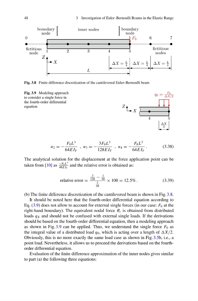
Fig. 3.8 Finite difference discretization of the cantilevered Euler–Bernoulli beam
Fig. 3.9 Modeling approach
to consider a single force in
the fourth-order differential
equation
u 2 = −
F 0 L
3
64E I Y
, u 3 = −
3F 0 L
3
128E I Y
, u 4 = −
F 0 L
3
64E I Y
.
(3.38)
The analytical solution for the displacement at the force application point can be
taken from [10] as
−F 0 L
3
48E I Y
and the relative error is obtained as:
relative error =
3
128
−
1
48
1
48
× 100 = 12.5% .
(3.39)
(b) The finite difference discretization of the cantilevered beam is shown in Fig. 3.8.
It should be noted here that the fourth-order differential equation according to
Eq. (3.9) does not allow to account for external single forces (in our case: F 0 at the
right-hand boundary). The equivalent nodal force R i is obtained from distributed
loads q X and should not be confused with external single loads. If the derivations
should be based on the fourth-order differential equation, then a modeling approach
as shown in Fig. 3.9 can be applied. Thus, we understand the single force F 0 as
the integral value of a distributed load q 0 , which is acting over a length of
Obviously, this is no more exactly the same load case as shown in Fig. 3.5b, i.e., a
point load. Nevertheless, it allows us to proceed the derivations based on the fourthorder differential equation.
Evaluation of the finite difference approximation of the inner nodes gives similar
to part (a) the following three equations:
3 Investigation of Euler–Bernoulli Beams in the Elastic Range
Fig. 3.8 Finite difference discretization of the cantilevered Euler–Bernoulli beam
Fig. 3.9 Modeling approach
to consider a single force in
the fourth-order differential
equation
u 2 = −
F 0 L
3
64E I Y
, u 3 = −
3F 0 L
3
128E I Y
, u 4 = −
F 0 L
3
64E I Y
.
(3.38)
The analytical solution for the displacement at the force application point can be
taken from [10] as
−F 0 L
3
48E I Y
and the relative error is obtained as:
relative error =
3
128
−
1
48
1
48
× 100 = 12.5% .
(3.39)
(b) The finite difference discretization of the cantilevered beam is shown in Fig. 3.8.
It should be noted here that the fourth-order differential equation according to
Eq. (3.9) does not allow to account for external single forces (in our case: F 0 at the
right-hand boundary). The equivalent nodal force R i is obtained from distributed
loads q X and should not be confused with external single loads. If the derivations
should be based on the fourth-order differential equation, then a modeling approach
as shown in Fig. 3.9 can be applied. Thus, we understand the single force F 0 as
the integral value of a distributed load q 0 , which is acting over a length of
Obviously, this is no more exactly the same load case as shown in Fig. 3.5b, i.e., a
point load. Nevertheless, it allows us to proceed the derivations based on the fourthorder differential equation.
Evaluation of the finite difference approximation of the inner nodes gives similar
to part (a) the following three equations: