

30
2 Investigation of Rods in the Elastic Range
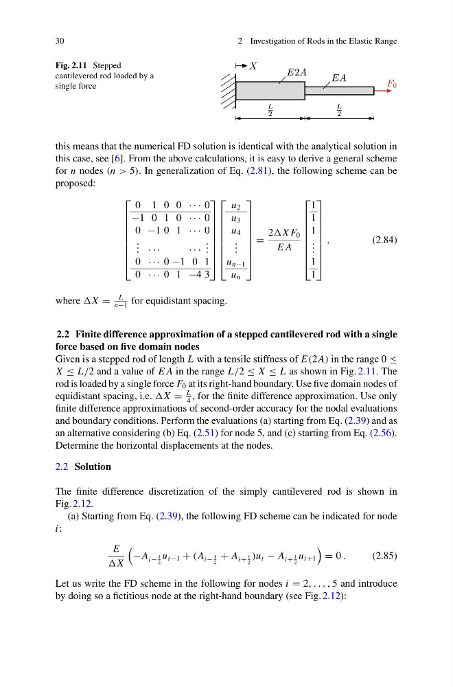
Fig. 2.11 Stepped
cantilevered rod loaded by a
single force
this means that the numerical FD solution is identical with the analytical solution in
this case, see [6]. From the above calculations, it is easy to derive a general scheme
for n nodes (n > 5). In generalization of Eq. (2.81), the following scheme can be
proposed:
⎡
⎢
⎢
⎢
⎢
⎢
⎢
⎢
⎣
0 1 0 0 · · · 0
−1 0 1 0 · · · 0
0 −1 0 1 · · · 0
. . . · · ·
· · ·
. . .
0 · · · 0 −1 0 1
0 · · · 0 1 −4 3
⎤
⎥
⎥
⎥
⎥
⎥
⎥
⎥
⎦
⎡
⎢
⎢
⎢
⎢
⎢
⎢
⎢
⎣
u 2
u 3
u 4
. . .
u n−1
u n
⎤
⎥
⎥
⎥
⎥
⎥
⎥
⎥
⎦
=
2X F 0
E A
⎡
⎢
⎢
⎢
⎢
⎢
⎢
⎢
⎣
1
1
1
. . .
1
1
⎤
⎥
⎥
⎥
⎥
⎥
⎥
⎥
⎦
,
(2.84)
where =
L
n−1
for equidistant spacing.
2.2 Finite difference approximation of a stepped cantilevered rod with a single
force based on five domain nodes
Given is a stepped rod of length L with a tensile stiffness of E(2 A) in the range 0 ≤
X ≤ L/2 and a value of E A in the range L/2 ≤ X ≤ L as shown in Fig. 2.11. The
rod is loaded by a single force F 0 at its right-hand boundary. Use five domain nodes of
equidistant spacing, i.e. =
L
4
, for the finite difference approximation. Use only
finite difference approximations of second-order accuracy for the nodal evaluations
and boundary conditions. Perform the evaluations (a) starting from Eq. (2.39) and as
an alternative considering (b) Eq. (2.51) for node 5, and (c) starting from Eq. (2.56).
Determine the horizontal displacements at the nodes.
2.2 Solution
The finite difference discretization of the simply cantilevered rod is shown in
Fig. 2.12.
(a) Starting from Eq. (2.39), the following FD scheme can be indicated for node
i:
E
−A i−
1
2
u i−1 + (A i−
1
2
+ A i+
1
2
)u i − A i+
1
2
u i+1
= 0 .
(2.85)
Let us write the FD scheme in the following for nodes i = 2, . . . , 5 and introduce
by doing so a fictitious node at the right-hand boundary (see Fig. 2.12):
2 Investigation of Rods in the Elastic Range
Fig. 2.11 Stepped
cantilevered rod loaded by a
single force
this means that the numerical FD solution is identical with the analytical solution in
this case, see [6]. From the above calculations, it is easy to derive a general scheme
for n nodes (n > 5). In generalization of Eq. (2.81), the following scheme can be
proposed:
⎡
⎢
⎢
⎢
⎢
⎢
⎢
⎢
⎣
0 1 0 0 · · · 0
−1 0 1 0 · · · 0
0 −1 0 1 · · · 0
. . . · · ·
· · ·
. . .
0 · · · 0 −1 0 1
0 · · · 0 1 −4 3
⎤
⎥
⎥
⎥
⎥
⎥
⎥
⎥
⎦
⎡
⎢
⎢
⎢
⎢
⎢
⎢
⎢
⎣
u 2
u 3
u 4
. . .
u n−1
u n
⎤
⎥
⎥
⎥
⎥
⎥
⎥
⎥
⎦
=
2X F 0
E A
⎡
⎢
⎢
⎢
⎢
⎢
⎢
⎢
⎣
1
1
1
. . .
1
1
⎤
⎥
⎥
⎥
⎥
⎥
⎥
⎥
⎦
,
(2.84)
where =
L
n−1
for equidistant spacing.
2.2 Finite difference approximation of a stepped cantilevered rod with a single
force based on five domain nodes
Given is a stepped rod of length L with a tensile stiffness of E(2 A) in the range 0 ≤
X ≤ L/2 and a value of E A in the range L/2 ≤ X ≤ L as shown in Fig. 2.11. The
rod is loaded by a single force F 0 at its right-hand boundary. Use five domain nodes of
equidistant spacing, i.e. =
L
4
, for the finite difference approximation. Use only
finite difference approximations of second-order accuracy for the nodal evaluations
and boundary conditions. Perform the evaluations (a) starting from Eq. (2.39) and as
an alternative considering (b) Eq. (2.51) for node 5, and (c) starting from Eq. (2.56).
Determine the horizontal displacements at the nodes.
2.2 Solution
The finite difference discretization of the simply cantilevered rod is shown in
Fig. 2.12.
(a) Starting from Eq. (2.39), the following FD scheme can be indicated for node
i:
E
−A i−
1
2
u i−1 + (A i−
1
2
+ A i+
1
2
)u i − A i+
1
2
u i+1
= 0 .
(2.85)
Let us write the FD scheme in the following for nodes i = 2, . . . , 5 and introduce
by doing so a fictitious node at the right-hand boundary (see Fig. 2.12):