

2.3 Varying Material and Geometry Parameters
19
A finite difference approximation of this equation can be introduced in different
ways. Let us first neglect for simplicity the distributed load ( p(X ) = 0) since the
treatment of a distributed load is discussed in Sect. 2.2.
The first approach is based on the introduction of an auxiliary function v(x) of
the form:
v(X ) = k(X )
du
dX
.
(2.34)
Thus, the differential equation (2.33) can be expressed in a much more simpler way
under the simplification that the distributed load is neglected as:
dv(X )
dX
= 0 .
(2.35)
The first task is now to approximate the first-order derivative
dv
dX
. To this end, let us
consider the centered difference expression from Table 1.1 and replace by
2
.
Thus, the centered difference approximation is given by
dv(X )
dX
i
=
v i+
1
2
− v i−
1
2
,
(2.36)
where, for example, the notation ‘i +
1
2
’ refers to the value of the function v in the
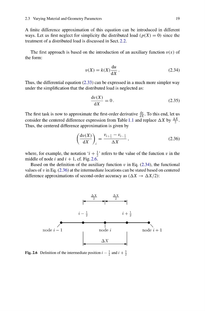
middle of node i and i + 1, cf. Fig. 2.6.
Based on the definition of the auxiliary function v in Eq. (2.34), the functional
values of v in Eq. (2.36) at the intermediate locations can be stated based on centered
difference approximations of second-order accuracy as ((X →
Fig. 2.6 Definition of the intermediate position i −
1
2 and i +
1
2
19
A finite difference approximation of this equation can be introduced in different
ways. Let us first neglect for simplicity the distributed load ( p(X ) = 0) since the
treatment of a distributed load is discussed in Sect. 2.2.
The first approach is based on the introduction of an auxiliary function v(x) of
the form:
v(X ) = k(X )
du
dX
.
(2.34)
Thus, the differential equation (2.33) can be expressed in a much more simpler way
under the simplification that the distributed load is neglected as:
dv(X )
dX
= 0 .
(2.35)
The first task is now to approximate the first-order derivative
dv
dX
. To this end, let us
consider the centered difference expression from Table 1.1 and replace by
2
.
Thus, the centered difference approximation is given by
dv(X )
dX
i
=
v i+
1
2
− v i−
1
2
,
(2.36)
where, for example, the notation ‘i +
1
2
’ refers to the value of the function v in the
middle of node i and i + 1, cf. Fig. 2.6.
Based on the definition of the auxiliary function v in Eq. (2.34), the functional
values of v in Eq. (2.36) at the intermediate locations can be stated based on centered
difference approximations of second-order accuracy as ((X →
Fig. 2.6 Definition of the intermediate position i −
1
2 and i +
1
2