

18
2 Investigation of Rods in the Elastic Range
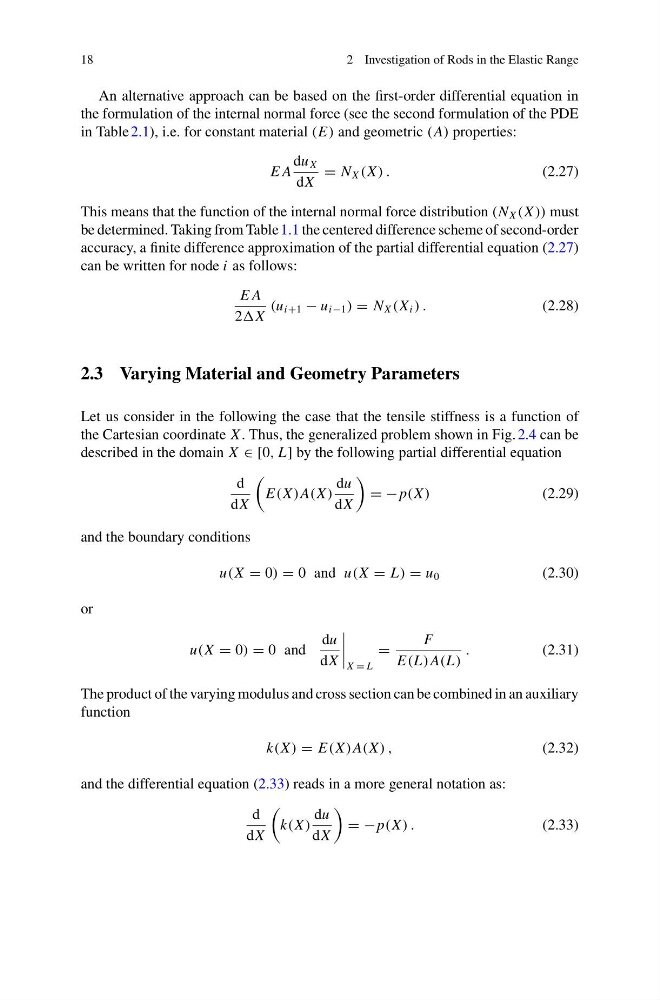
An alternative approach can be based on the first-order differential equation in
the formulation of the internal normal force (see the second formulation of the PDE
in Table 2.1), i.e. for constant material (E) and geometric (A) properties:
E A
du X
dX
= N X (X ) .
(2.27)
This means that the function of the internal normal force distribution (N X (X )) must
be determined. Taking from Table 1.1 the centered difference scheme of second-order
accuracy, a finite difference approximation of the partial differential equation (2.27)
can be written for node i as follows:
E A
2X
(u i+1 − u i−1 ) = N X (X i ) .
(2.28)
2.3 Varying Material and Geometry Parameters
Let us consider in the following the case that the tensile stiffness is a function of
the Cartesian coordinate X . Thus, the generalized problem shown in Fig. 2.4 can be
described in the domain X ∈ [0, L] by the following partial differential equation
d
dX
E(X )A(X )
du
dX
= −p(X )
(2.29)
and the boundary conditions
u(X = 0) = 0 and u(X = L) = u 0
(2.30)
or
u(X = 0) = 0 and
du
dX
X = L
=
F
E(L)A(L)
.
(2.31)
The product of the varying modulus and cross section can be combined in an auxiliary
function
k(X ) = E(X )A(X ) ,
(2.32)
and the differential equation (2.33) reads in a more general notation as:
d
dX
k(X )
du
dX
= −p(X ) .
(2.33)
2 Investigation of Rods in the Elastic Range
An alternative approach can be based on the first-order differential equation in
the formulation of the internal normal force (see the second formulation of the PDE
in Table 2.1), i.e. for constant material (E) and geometric (A) properties:
E A
du X
dX
= N X (X ) .
(2.27)
This means that the function of the internal normal force distribution (N X (X )) must
be determined. Taking from Table 1.1 the centered difference scheme of second-order
accuracy, a finite difference approximation of the partial differential equation (2.27)
can be written for node i as follows:
E A
2X
(u i+1 − u i−1 ) = N X (X i ) .
(2.28)
2.3 Varying Material and Geometry Parameters
Let us consider in the following the case that the tensile stiffness is a function of
the Cartesian coordinate X . Thus, the generalized problem shown in Fig. 2.4 can be
described in the domain X ∈ [0, L] by the following partial differential equation
d
dX
E(X )A(X )
du
dX
= −p(X )
(2.29)
and the boundary conditions
u(X = 0) = 0 and u(X = L) = u 0
(2.30)
or
u(X = 0) = 0 and
du
dX
X = L
=
F
E(L)A(L)
.
(2.31)
The product of the varying modulus and cross section can be combined in an auxiliary
function
k(X ) = E(X )A(X ) ,
(2.32)
and the differential equation (2.33) reads in a more general notation as:
d
dX
k(X )
du
dX
= −p(X ) .
(2.33)