

10
1 Mathematical Physics
Poisson distribution
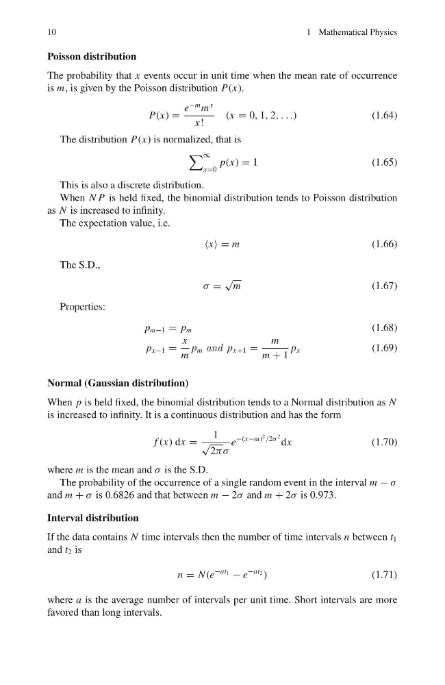
The probability that x events occur in unit time when the mean rate of occurrence
is m, is given by the Poisson distribution P(x).
P(x) =
e
−m m
x
x!
(x = 0, 1, 2, . . .)
(1.64)
The distribution P(x) is normalized, that is
∞
x=0
p(x) = 1
(1.65)
This is also a discrete distribution.
When N P is held fixed, the binomial distribution tends to Poisson distribution
as N is increased to infinity.
The expectation value, i.e.
x = m
(1.66)
The S.D.,
σ =
√
m
(1.67)
Properties:
p m−1 = p m
(1.68)
p x−1 =
x
m
p m and p x+1 =
m
m + 1
p x
(1.69)
Normal (Gaussian distribution)
When p is held fixed, the binomial distribution tends to a Normal distribution as N
is increased to infinity. It is a continuous distribution and has the form
f (x) dx =
1
√
2πσ
e
−(x−m)
2 /2σ
2 dx
(1.70)
where m is the mean and σ is the S.D.
The probability of the occurrence of a single random event in the interval m − σ
and m + σ is 0.6826 and that between m − 2σ and m + 2σ is 0.973.
Interval distribution
If the data contains N time intervals then the number of time intervals n between t 1
and t 2 is
n = N (e
−at1
− e
−at2 )
(1.71)
where a is the average number of intervals per unit time. Short intervals are more
favored than long intervals.
1 Mathematical Physics
Poisson distribution
The probability that x events occur in unit time when the mean rate of occurrence
is m, is given by the Poisson distribution P(x).
P(x) =
e
−m m
x
x!
(x = 0, 1, 2, . . .)
(1.64)
The distribution P(x) is normalized, that is
∞
x=0
p(x) = 1
(1.65)
This is also a discrete distribution.
When N P is held fixed, the binomial distribution tends to Poisson distribution
as N is increased to infinity.
The expectation value, i.e.
x = m
(1.66)
The S.D.,
σ =
√
m
(1.67)
Properties:
p m−1 = p m
(1.68)
p x−1 =
x
m
p m and p x+1 =
m
m + 1
p x
(1.69)
Normal (Gaussian distribution)
When p is held fixed, the binomial distribution tends to a Normal distribution as N
is increased to infinity. It is a continuous distribution and has the form
f (x) dx =
1
√
2πσ
e
−(x−m)
2 /2σ
2 dx
(1.70)
where m is the mean and σ is the S.D.
The probability of the occurrence of a single random event in the interval m − σ
and m + σ is 0.6826 and that between m − 2σ and m + 2σ is 0.973.
Interval distribution
If the data contains N time intervals then the number of time intervals n between t 1
and t 2 is
n = N (e
−at1
− e
−at2 )
(1.71)
where a is the average number of intervals per unit time. Short intervals are more
favored than long intervals.