

200
3 Quantum Mechanics – II
3.52 u 0 =
α
√
π
e
−ξ
2 /2 H 0 (ξ ); ξ = αx
P = 1 −
a
−a
|u 0 |
2 dx = 1 − 2
a
0
(α/
√
π)e
−ξ
2 /2 dx
= 1 −
2
√
π
aα
0
e
−ξ
2 dξ
E 0 =
1
/ 2 ka
2
=
ω
2
(n = 0)
Therefore a
2
=
ω
k
=
k
k
m
1/2 =
√
km
=
1
α 2
Therefore α
2 a
2
= 1 or αa = 1
P = 1 −
2
√
π
1
0
e
−ξ 2 dξ
= 1 −
2
√
π
1 − ξ
2
+
ξ
4
2!
−
ξ
6
3!
+
ξ
8
4!
dξ
= 1 −
2
√
π
1 −
1
3
+
1
10
−
1
42
+
1
216
. . .
≈ 0.16
Therefore, p ≈ 16%
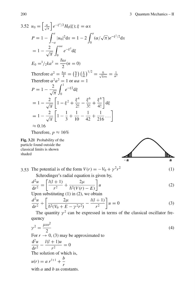
Fig. 3.21 Probability of the
particle found outside the
classical limits is shown
shaded
3.53 The potential is of the form V (r ) = −V 0 + γ
2 r
2
(1)
Schrodinger’s radial equation is given by,
d
2 u
dr 2 =
l(l + 1)
r 2 +
2μ
2 (V (r ) − E)
u
(2)
Upon substituting (1) in (2), we obtain
d
2 u
dr 2 +
2μ
2 (V 0 + E − γ 2 r 2 )
−
l(l + 1)
r 2
u = 0
( 3 )
The quantity γ
2 can be expressed in terms of the classical oscillator frequency
γ
2
=
μω
2
2
(4)
For r → 0, (3) may be approximated to
d
2 u
dr 2 −
l(l + 1)u
r 2
= 0
The solution of which is,
u(r ) = a r
l+1
+
b
r
with a and b as constants.
3 Quantum Mechanics – II
3.52 u 0 =
α
√
π
e
−ξ
2 /2 H 0 (ξ ); ξ = αx
P = 1 −
a
−a
|u 0 |
2 dx = 1 − 2
a
0
(α/
√
π)e
−ξ
2 /2 dx
= 1 −
2
√
π
aα
0
e
−ξ
2 dξ
E 0 =
1
/ 2 ka
2
=
ω
2
(n = 0)
Therefore a
2
=
ω
k
=
k
k
m
1/2 =
√
km
=
1
α 2
Therefore α
2 a
2
= 1 or αa = 1
P = 1 −
2
√
π
1
0
e
−ξ 2 dξ
= 1 −
2
√
π
1 − ξ
2
+
ξ
4
2!
−
ξ
6
3!
+
ξ
8
4!
dξ
= 1 −
2
√
π
1 −
1
3
+
1
10
−
1
42
+
1
216
. . .
≈ 0.16
Therefore, p ≈ 16%
Fig. 3.21 Probability of the
particle found outside the
classical limits is shown
shaded
3.53 The potential is of the form V (r ) = −V 0 + γ
2 r
2
(1)
Schrodinger’s radial equation is given by,
d
2 u
dr 2 =
l(l + 1)
r 2 +
2μ
2 (V (r ) − E)
u
(2)
Upon substituting (1) in (2), we obtain
d
2 u
dr 2 +
2μ
2 (V 0 + E − γ 2 r 2 )
−
l(l + 1)
r 2
u = 0
( 3 )
The quantity γ
2 can be expressed in terms of the classical oscillator frequency
γ
2
=
μω
2
2
(4)
For r → 0, (3) may be approximated to
d
2 u
dr 2 −
l(l + 1)u
r 2
= 0
The solution of which is,
u(r ) = a r
l+1
+
b
r
with a and b as constants.