

176
3 Quantum Mechanics – II
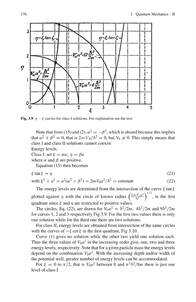
Fig. 3.9 η − ξ curves for class I solutions. For explanation see the text
Note that from (15) and (2), α
2
= −β
2 , which is absurd because this implies
that α
2
+ β
2
= 0, that is 2mV 0 /
2
= 0, but V 0 = 0. This simply means that
class I and class II solutions cannot coexist
Energy levels:
Class I: set ξ = αa; η = βa
where α and β are positive.
Equation (15) then becomes
ξ tan ξ = η
(21)
with ξ
2
+ η
2
= a
2 (α
2
+ β
2 ) = 2mV 0 a
2
/
2
= constant
(22)
The energy levels are determined from the intersection of the curve ξ tan ξ
plotted against η with the circle of known radius
2mV 0 a
2
2
1/2
, in the first
quadrant since ξ and η are restricted to positive values.
The circles, Eq. (22), are drawn for V 0 a
2
=
2
/2m, 4
2
/2m and 9
2
/2m
for curves 1, 2 and 3 respectively Fig 3.9. For the first two values there is only
one solution while for the third one there are two solutions.
For class II, energy levels are obtained from intersection of the same circles
with the curves of −ξ cot ξ in the first quadrant, Fig 3.10.
Curve (1) gives no solution while the other two yield one solution each.
Thus the three values of V 0 a
2 in the increasing order give, one, two and three
energy levels, respectively. Note that for a given particle mass the energy levels
depend on the combination V 0 a
2 . With the increasing depth and/or width of
the potential well, greater number of energy levels can be accommodated.
For ξ = 0 to π/2, that is V 0 a
2 between 0 and π
2
2
/8m there is just one
level of class I
3 Quantum Mechanics – II
Fig. 3.9 η − ξ curves for class I solutions. For explanation see the text
Note that from (15) and (2), α
2
= −β
2 , which is absurd because this implies
that α
2
+ β
2
= 0, that is 2mV 0 /
2
= 0, but V 0 = 0. This simply means that
class I and class II solutions cannot coexist
Energy levels:
Class I: set ξ = αa; η = βa
where α and β are positive.
Equation (15) then becomes
ξ tan ξ = η
(21)
with ξ
2
+ η
2
= a
2 (α
2
+ β
2 ) = 2mV 0 a
2
/
2
= constant
(22)
The energy levels are determined from the intersection of the curve ξ tan ξ
plotted against η with the circle of known radius
2mV 0 a
2
2
1/2
, in the first
quadrant since ξ and η are restricted to positive values.
The circles, Eq. (22), are drawn for V 0 a
2
=
2
/2m, 4
2
/2m and 9
2
/2m
for curves 1, 2 and 3 respectively Fig 3.9. For the first two values there is only
one solution while for the third one there are two solutions.
For class II, energy levels are obtained from intersection of the same circles
with the curves of −ξ cot ξ in the first quadrant, Fig 3.10.
Curve (1) gives no solution while the other two yield one solution each.
Thus the three values of V 0 a
2 in the increasing order give, one, two and three
energy levels, respectively. Note that for a given particle mass the energy levels
depend on the combination V 0 a
2 . With the increasing depth and/or width of
the potential well, greater number of energy levels can be accommodated.
For ξ = 0 to π/2, that is V 0 a
2 between 0 and π
2
2
/8m there is just one
level of class I