

162
3 Quantum Mechanics – II
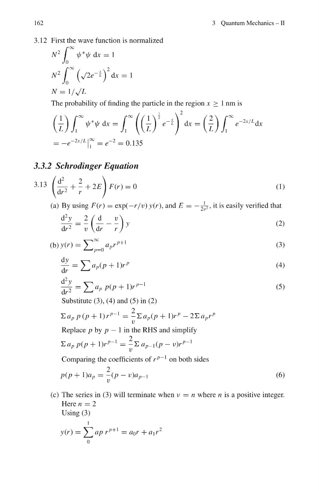
3.12 First the wave function is normalized
N
2
∞
0
ψ
∗
ψ dx = 1
N
2
∞
0
√
2e
−
x
L
2
dx = 1
N = 1/
√
L
The probability of finding the particle in the region x ≥ 1 nm is
1
L
∞
1
ψ
∗
ψ dx =
∞
1
1
L
1
2
e
−
x
L
2
dx =
2
L
∞
1
e
−2x/L dx
= −e
−2x/L
∞
1
= e
−2
= 0.135
3.3.2 Schrodinger Equation
3.13
d
2
dr 2 +
2
r
+ 2E
F(r ) = 0
( 1 )
(a) By using F(r ) = exp(−r/v) y(r ), and E = −
1
2ν 2 , it is easily verified that
d
2 y
dr 2 =
2
v
d
dr
−
v
r
y
(2)
(b) y(r ) =
∞
p=0
a p r
p+1
(3)
dy
dr
=
a p ( p + 1)r
p
(4)
d
2 y
dr 2 =
a p p( p + 1)r
p−1
(5)
Substitute (3), (4) and (5) in (2)
Σ a p p ( p + 1) r
p−1
=
2
v
Σ a p ( p + 1)r
p
− 2Σ a p r
p
Replace p by p − 1 in the RHS and simplify
Σ a p p( p + 1)r
p−1
=
2
v
Σ a p−1 ( p − ν)r
p−1
Comparing the coefficients of r
p−1 on both sides
p( p + 1)a p =
2
v
( p − v)a p−1
(6)
(c) The series in (3) will terminate when ν = n where n is a positive integer.
Here n = 2
Using (3)
y(r ) =
1
0
ap r
p+1
= a 0 r + a 1 r
2
3 Quantum Mechanics – II
3.12 First the wave function is normalized
N
2
∞
0
ψ
∗
ψ dx = 1
N
2
∞
0
√
2e
−
x
L
2
dx = 1
N = 1/
√
L
The probability of finding the particle in the region x ≥ 1 nm is
1
L
∞
1
ψ
∗
ψ dx =
∞
1
1
L
1
2
e
−
x
L
2
dx =
2
L
∞
1
e
−2x/L dx
= −e
−2x/L
∞
1
= e
−2
= 0.135
3.3.2 Schrodinger Equation
3.13
d
2
dr 2 +
2
r
+ 2E
F(r ) = 0
( 1 )
(a) By using F(r ) = exp(−r/v) y(r ), and E = −
1
2ν 2 , it is easily verified that
d
2 y
dr 2 =
2
v
d
dr
−
v
r
y
(2)
(b) y(r ) =
∞
p=0
a p r
p+1
(3)
dy
dr
=
a p ( p + 1)r
p
(4)
d
2 y
dr 2 =
a p p( p + 1)r
p−1
(5)
Substitute (3), (4) and (5) in (2)
Σ a p p ( p + 1) r
p−1
=
2
v
Σ a p ( p + 1)r
p
− 2Σ a p r
p
Replace p by p − 1 in the RHS and simplify
Σ a p p( p + 1)r
p−1
=
2
v
Σ a p−1 ( p − ν)r
p−1
Comparing the coefficients of r
p−1 on both sides
p( p + 1)a p =
2
v
( p − v)a p−1
(6)
(c) The series in (3) will terminate when ν = n where n is a positive integer.
Here n = 2
Using (3)
y(r ) =
1
0
ap r
p+1
= a 0 r + a 1 r
2