

22
ATOMIC STRUCTURE AND BONDING
x
y
z
1s
2s
2p y
2p x
2p z
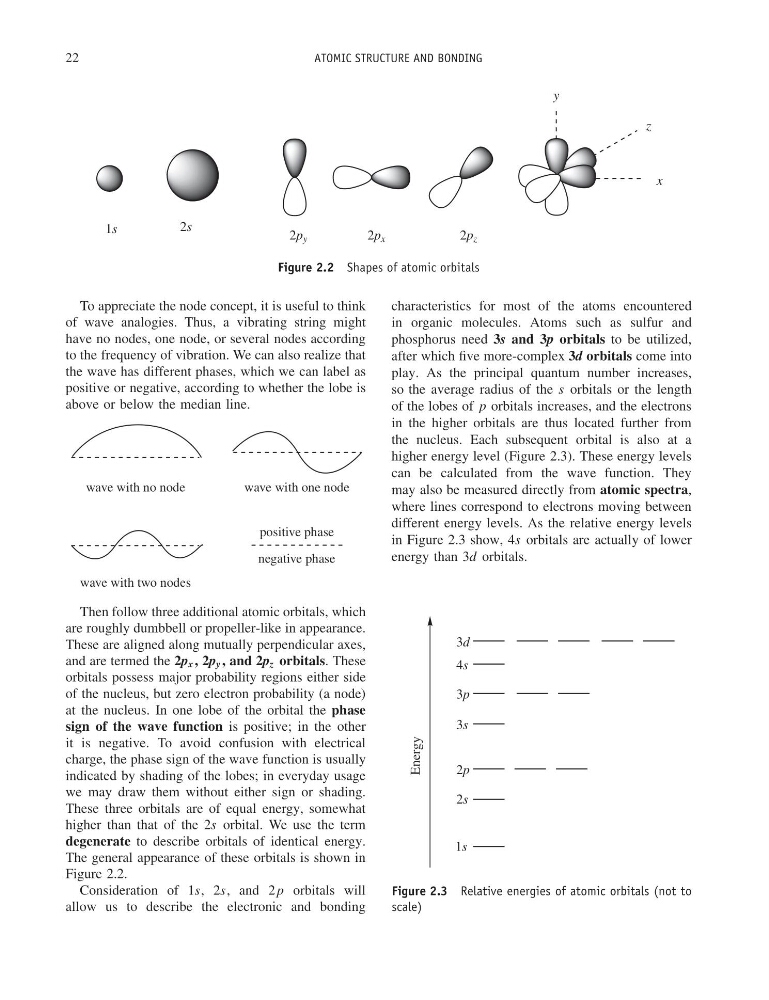
Figure 2.2 Shapes of atomic orbitals
To appreciate the node concept, it is useful to think
of wave analogies. Thus, a vibrating string might
have no nodes, one node, or several nodes according
to the frequency of vibration. We can also realize that
the wave has different phases, which we can label as
positive or negative, according to whether the lobe is
above or below the median line.
wave with no node
wave with one node
wave with two nodes
positive phase
negative phase
Then follow three additional atomic orbitals, which
are roughly dumbbell or propeller-like in appearance.
These are aligned along mutually perpendicular axes,
and are termed the 2p x , 2p y , and 2p z orbitals. These
orbitals possess major probability regions either side
of the nucleus, but zero electron probability (a node)
at the nucleus. In one lobe of the orbital the phase
sign of the wave function is positive; in the other
it is negative. To avoid confusion with electrical
charge, the phase sign of the wave function is usually
indicated by shading of the lobes; in everyday usage
we may draw them without either sign or shading.
These three orbitals are of equal energy, somewhat
higher than that of the 2s orbital. We use the term
degenerate to describe orbitals of identical energy.
The general appearance of these orbitals is shown in
Figure 2.2.
Consideration of 1s, 2s, and 2p orbitals will
allow us to describe the electronic and bonding
characteristics for most of the atoms encountered
in organic molecules. Atoms such as sulfur and
phosphorus need 3s and 3p orbitals to be utilized,
after which five more-complex 3d orbitals come into
play. As the principal quantum number increases,
so the average radius of the s orbitals or the length
of the lobes of p orbitals increases, and the electrons
in the higher orbitals are thus located further from
the nucleus. Each subsequent orbital is also at a
higher energy level (Figure 2.3). These energy levels
can be calculated from the wave function. They
may also be measured directly from atomic spectra,
where lines correspond to electrons moving between
different energy levels. As the relative energy levels
in Figure 2.3 show, 4s orbitals are actually of lower
energy than 3d orbitals.
Energy
1s
2s
2p
3s
3p
3d
4s
Figure 2.3 Relative energies of atomic orbitals (not to
scale)
ATOMIC STRUCTURE AND BONDING
x
y
z
1s
2s
2p y
2p x
2p z
Figure 2.2 Shapes of atomic orbitals
To appreciate the node concept, it is useful to think
of wave analogies. Thus, a vibrating string might
have no nodes, one node, or several nodes according
to the frequency of vibration. We can also realize that
the wave has different phases, which we can label as
positive or negative, according to whether the lobe is
above or below the median line.
wave with no node
wave with one node
wave with two nodes
positive phase
negative phase
Then follow three additional atomic orbitals, which
are roughly dumbbell or propeller-like in appearance.
These are aligned along mutually perpendicular axes,
and are termed the 2p x , 2p y , and 2p z orbitals. These
orbitals possess major probability regions either side
of the nucleus, but zero electron probability (a node)
at the nucleus. In one lobe of the orbital the phase
sign of the wave function is positive; in the other
it is negative. To avoid confusion with electrical
charge, the phase sign of the wave function is usually
indicated by shading of the lobes; in everyday usage
we may draw them without either sign or shading.
These three orbitals are of equal energy, somewhat
higher than that of the 2s orbital. We use the term
degenerate to describe orbitals of identical energy.
The general appearance of these orbitals is shown in
Figure 2.2.
Consideration of 1s, 2s, and 2p orbitals will
allow us to describe the electronic and bonding
characteristics for most of the atoms encountered
in organic molecules. Atoms such as sulfur and
phosphorus need 3s and 3p orbitals to be utilized,
after which five more-complex 3d orbitals come into
play. As the principal quantum number increases,
so the average radius of the s orbitals or the length
of the lobes of p orbitals increases, and the electrons
in the higher orbitals are thus located further from
the nucleus. Each subsequent orbital is also at a
higher energy level (Figure 2.3). These energy levels
can be calculated from the wave function. They
may also be measured directly from atomic spectra,
where lines correspond to electrons moving between
different energy levels. As the relative energy levels
in Figure 2.3 show, 4s orbitals are actually of lower
energy than 3d orbitals.
Energy
1s
2s
2p
3s
3p
3d
4s
Figure 2.3 Relative energies of atomic orbitals (not to
scale)