

74
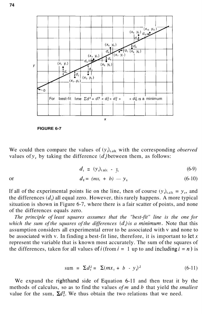
For best-fit line Ed
2 = d? + dj + d3
2 +
+ d,
2
0 is a minimum
FIGURE 6-7
We could then compare the values of (y^ait with the corresponding observed
values of y, by taking the difference (d) between them, as follows:
or
d, = (y,)cak - y,
d ( = (mx, + b) — y t
(6-9)
(6-10)
If all of the experimental points lie on the line, then of course (y,) tdk = y,, and
the differences (J,) all equal zero. However, this rarely happens. A more typical
situation is shown in Figure 6-7, where there is a fair scatter of points, and none
of the differences equals zero.
The principle of least squares assumes that the "best-fit" line is the one for
which the sum of the squares of the differences (d,) is a minimum. Note that this
assumption considers all experimental error to be associated with v and none to
be associated with v. In finding a best-fit line, therefore, it is important to let,v
represent the variable that is known most accurately. The sum of the squares of
the differences, taken for all values of/ (from / = 1 up to and including;' = n) is
sum = Srff = "Z(mx, + b - y)
2
(6-11)
We expand the righthand side of Equation 6-11 and then treat it by the
methods of calculus, so as to find the values of m and b that yield the smallest
value for the sum, Sdjr. We thus obtain the two relations that we need.
For best-fit line Ed
2 = d? + dj + d3
2 +
+ d,
2
0 is a minimum
FIGURE 6-7
We could then compare the values of (y^ait with the corresponding observed
values of y, by taking the difference (d) between them, as follows:
or
d, = (y,)cak - y,
d ( = (mx, + b) — y t
(6-9)
(6-10)
If all of the experimental points lie on the line, then of course (y,) tdk = y,, and
the differences (J,) all equal zero. However, this rarely happens. A more typical
situation is shown in Figure 6-7, where there is a fair scatter of points, and none
of the differences equals zero.
The principle of least squares assumes that the "best-fit" line is the one for
which the sum of the squares of the differences (d,) is a minimum. Note that this
assumption considers all experimental error to be associated with v and none to
be associated with v. In finding a best-fit line, therefore, it is important to let,v
represent the variable that is known most accurately. The sum of the squares of
the differences, taken for all values of/ (from / = 1 up to and including;' = n) is
sum = Srff = "Z(mx, + b - y)
2
(6-11)
We expand the righthand side of Equation 6-11 and then treat it by the
methods of calculus, so as to find the values of m and b that yield the smallest
value for the sum, Sdjr. We thus obtain the two relations that we need.