

73
900
BOO
700
600
500
400
300
200
100
90
80
70
60
50
40
30
20
10
\
\
\
\
\
0.
\
T\
333I
1..
-0
\
___\
000150 h
\
V
\
\ \ v \ \
V \
27
2.8
29
3.0
3.1
3.2
33
7
X1 °
3
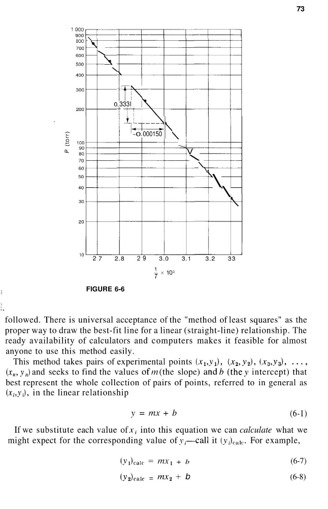
FIGURE 6-6
followed. There is universal acceptance of the "method of least squares" as the
proper way to draw the best-fit line for a linear (straight-line) relationship. The
ready availability of calculators and computers makes it feasible for almost
anyone to use this method easily.
This method takes pairs of experimental points (x^, y^, (x 2 , y 2 ), (x a , y^, ...,
(x,,,y,,) and seeks to find the values ofm (the slope) and/? (they intercept) that
best represent the whole collection of pairs of points, referred to in general as
(x,, y,), in the linear relationship
y = mx + b
(6-1)
If we substitute each value of x, into this equation we can calculate what we
might expect for the corresponding value of y,—call it (y,) ca i t . For example,
(y 2 )caic =
i + b
b
(6-7)
(6-8)
900
BOO
700
600
500
400
300
200
100
90
80
70
60
50
40
30
20
10
\
\
\
\
\
0.
\
T\
333I
1..
-0
\
___\
000150 h
\
V
\
\ \ v \ \
V \
27
2.8
29
3.0
3.1
3.2
33
7
X1 °
3
FIGURE 6-6
followed. There is universal acceptance of the "method of least squares" as the
proper way to draw the best-fit line for a linear (straight-line) relationship. The
ready availability of calculators and computers makes it feasible for almost
anyone to use this method easily.
This method takes pairs of experimental points (x^, y^, (x 2 , y 2 ), (x a , y^, ...,
(x,,,y,,) and seeks to find the values ofm (the slope) and/? (they intercept) that
best represent the whole collection of pairs of points, referred to in general as
(x,, y,), in the linear relationship
y = mx + b
(6-1)
If we substitute each value of x, into this equation we can calculate what we
might expect for the corresponding value of y,—call it (y,) ca i t . For example,
(y 2 )caic =
i + b
b
(6-7)
(6-8)