

235
1
[A]
1
[A]
2
y intercept = [A] 0
"y intercept =
f
(a)
(
(b)
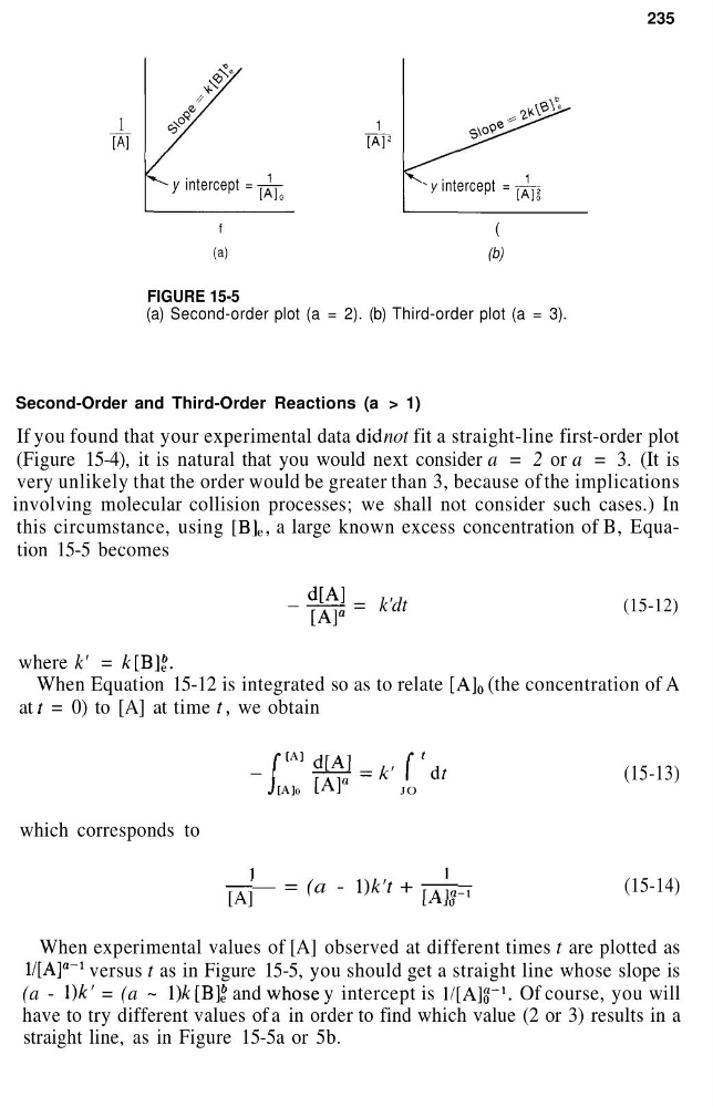
FIGURE 15-5
(a) Second-order plot (a = 2). (b) Third-order plot (a = 3).
Second-Order and Third-Order Reactions (a > 1)
If you found that your experimental data did not fit a straight-line first-order plot
(Figure 15-4), it is natural that you would next consider a = 2 or a = 3. (It is
very unlikely that the order would be greater than 3, because of the implications
involving molecular collision processes; we shall not consider such cases.) In
this circumstance, using [B] e , a large known excess concentration of B, Equation 15-5 becomes
d[A]
[A]"
= k'dt
(15-12)
where k' = k[B]l.
When Equation 15-12 is integrated so as to relate [A] 0 (the concentration of A
at / = 0) to [A] at time t, we obtain
which corresponds to
[A]
f
(A 'd[A] f
TA~^
= k
J[A]o L
A J
JO
— = (a - 1)A:V + 77^
(15-13)
(15-14)
When experimental values of [A] observed at different times t are plotted as
1/tA]""
1 versus t as in Figure 15-5, you should get a straight line whose slope is
(a - 1)A:' = (a ~ 1)A:[B]* and whose y intercept is l/[A]g
-1 . Of course, you will
have to try different values of a in order to find which value (2 or 3) results in a
straight line, as in Figure 15-5a or 5b.
1
[A]
1
[A]
2
y intercept = [A] 0
"y intercept =
f
(a)
(
(b)
FIGURE 15-5
(a) Second-order plot (a = 2). (b) Third-order plot (a = 3).
Second-Order and Third-Order Reactions (a > 1)
If you found that your experimental data did not fit a straight-line first-order plot
(Figure 15-4), it is natural that you would next consider a = 2 or a = 3. (It is
very unlikely that the order would be greater than 3, because of the implications
involving molecular collision processes; we shall not consider such cases.) In
this circumstance, using [B] e , a large known excess concentration of B, Equation 15-5 becomes
d[A]
[A]"
= k'dt
(15-12)
where k' = k[B]l.
When Equation 15-12 is integrated so as to relate [A] 0 (the concentration of A
at / = 0) to [A] at time t, we obtain
which corresponds to
[A]
f
(A 'd[A] f
TA~^
= k
J[A]o L
A J
JO
— = (a - 1)A:V + 77^
(15-13)
(15-14)
When experimental values of [A] observed at different times t are plotted as
1/tA]""
1 versus t as in Figure 15-5, you should get a straight line whose slope is
(a - 1)A:' = (a ~ 1)A:[B]* and whose y intercept is l/[A]g
-1 . Of course, you will
have to try different values of a in order to find which value (2 or 3) results in a
straight line, as in Figure 15-5a or 5b.