

387
Answers
601–700
Answers and Explanations
636.
4
15
Recall that the area A of the region bounded by the curves y = f
(x) and y = g(x) and by
the lines x = a and x = b, where f and g are continuous and f
(x) ≥ g(x) for all x in [a, b], is
A
f x g x dx
a
b
=
−
(
)
∫ ( ) ( )
More generically, in terms of a graph, you can think of the formula as
d
A
x
a
b
=
−
)
(
∫ (
) (
)
top function
bottom function
Note that lines x = a and x = b may not be given, so the limits of integration often correspond to points of intersection of the functions.
Begin by finding the points of intersection by setting the functions equal to each other
and solving for x:
x
x
x
x
x x
x
4
2
4
2
2
2
0
1 0
0 1
=
−
=
−
(
) =
= ±
,
Because x
2
≥ x
4
on the interval [–1, 1], the integral to find the area is
x
x dx
2
4
1
1
−
(
)
−
∫
The integrand is an even function, so it’s symmetric about the y-axis; therefore, you
can instead integrate on the interval [0, 1] and multiply by 2:
x
x dx
x
x dx
2
4
1
1
2
4
0
1
2
−
(
) =
−
(
)
−
∫
∫
This gives you the following:
2
2
3
5
2 1
3
1
5
4
15
2
4
0
1
3
5
0
1
x
x dx
x
x
−
(
) =
−
=
−
( ) =
∫
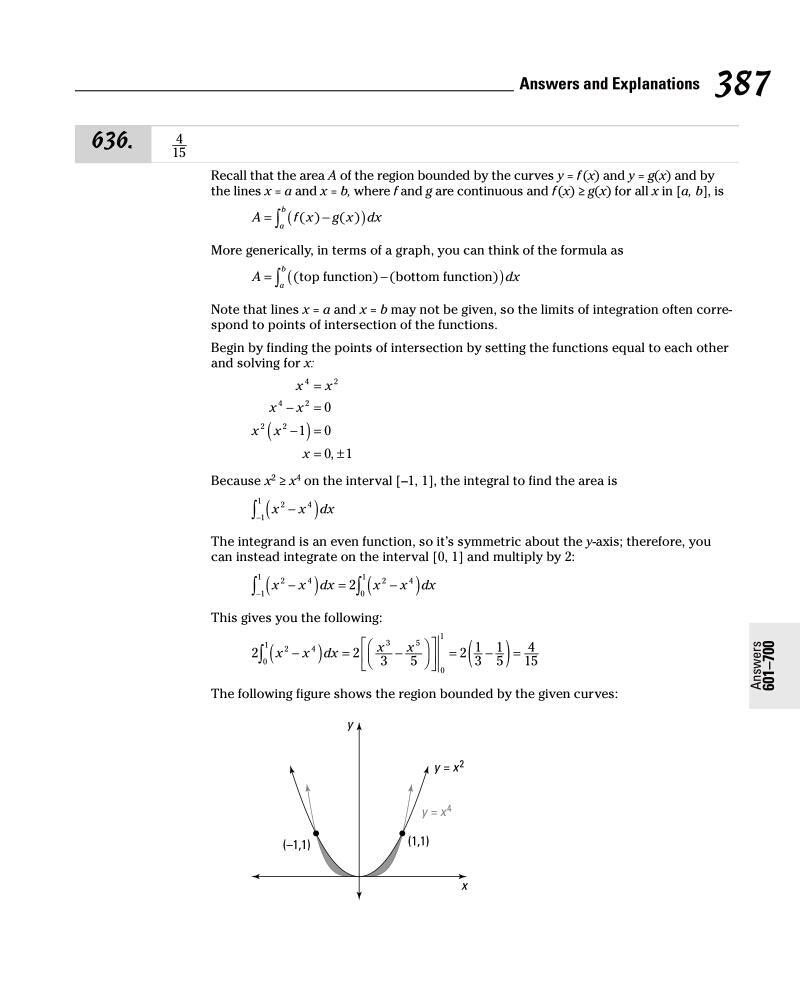
The following figure shows the region bounded by the given curves:
Answers
601–700
Answers and Explanations
636.
4
15
Recall that the area A of the region bounded by the curves y = f
(x) and y = g(x) and by
the lines x = a and x = b, where f and g are continuous and f
(x) ≥ g(x) for all x in [a, b], is
A
f x g x dx
a
b
=
−
(
)
∫ ( ) ( )
More generically, in terms of a graph, you can think of the formula as
d
A
x
a
b
=
−
)
(
∫ (
) (
)
top function
bottom function
Note that lines x = a and x = b may not be given, so the limits of integration often correspond to points of intersection of the functions.
Begin by finding the points of intersection by setting the functions equal to each other
and solving for x:
x
x
x
x
x x
x
4
2
4
2
2
2
0
1 0
0 1
=
−
=
−
(
) =
= ±
,
Because x
2
≥ x
4
on the interval [–1, 1], the integral to find the area is
x
x dx
2
4
1
1
−
(
)
−
∫
The integrand is an even function, so it’s symmetric about the y-axis; therefore, you
can instead integrate on the interval [0, 1] and multiply by 2:
x
x dx
x
x dx
2
4
1
1
2
4
0
1
2
−
(
) =
−
(
)
−
∫
∫
This gives you the following:
2
2
3
5
2 1
3
1
5
4
15
2
4
0
1
3
5
0
1
x
x dx
x
x
−
(
) =
−
=
−
( ) =
∫
The following figure shows the region bounded by the given curves: