

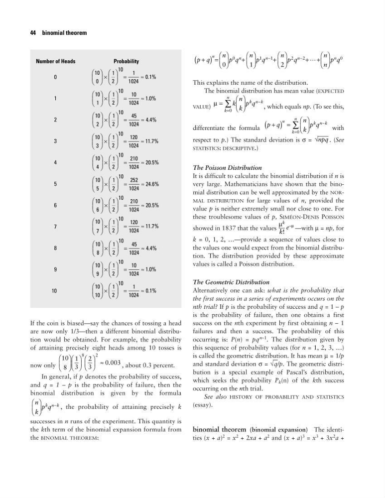
If the coin is biased—say the chances of tossing a head
are now only 1/3—then a different binomial distribution would be obtained. For example, the probability
of attaining precisely eight heads among 10 tosses is
now only
, about 0.3 percent.
In general, if p denotes the probability of success,
and q = 1 – p is the probability of failure, then the
binomial distribution is given by the formula
, the probability of attaining precisely k
successes in n runs of the experiment. This quantity is
the kth term of the binomial expansion formula from
the BINOMIAL THEOREM:
This explains the name of the distribution.
The binomial distribution has mean value (EXPECTED
VALUE)
, which equals np. (To see this,
differentiate the formula
with
respect to p.) The standard deviation is σ =
. (See
STATISTICS: DESCRIPTIVE.)
The Poisson Distribution
It is difficult to calculate the binomial distribution if n is
very large. Mathematicians have shown that the binomial distribution can be well approximated by the NORMAL DISTRIBUTION for large values of n, provided the
value p is neither extremely small nor close to one. For
these troublesome values of p, SIMÉON-DENIS POISSON
showed in 1837 that the values
—with µ = np, for
k = 0, 1, 2, …—provide a sequence of values close to
the values one would expect from the binomial distribution. The distribution provided by these approximate
values is called a Poisson distribution.
The Geometric Distribution
Alternatively one can ask: what is the probability that
the first success in a series of experiments occurs on the
nth trial? If p is the probability of success and q = 1 – p
is the probability of failure, then one obtains a first
success on the nth experiment by first obtaining n – 1
failures and then a success. The probability of this
occurring is: P(n) = pq
n–1
. The distribution given by
this sequence of probability values (for n = 1, 2, 3, …)
is called the geometric distribution. It has mean µ = 1/p
and standard deviation σ = √
–
q/p. The geometric distribution is a special example of Pascal’s distribution,
which seeks the probability P k (n) of the kth success
occurring on the nth trial.
See also HISTORY OF PROBABILITY AND STATISTICS
(essay).
binomial theorem (binomial expansion) The identities (x + a)
2 = x
2 + 2xa + a
2 and (x + a)
3 = x
3 + 3x
2
a +
µ
k
k!
e
–µ
√npq
p q
n
k
p q
n
k n k
k
n
+
( ) =
−
=
∑
0
µ =
−
=
∑ k
n
k
p q
k n k
k
n
0
p q
n p q
n p q
n p q
n
n
p q
n
n
n
n
n
+
( ) =
+
+
+ +
−
−
0
1
2
0
1
1
2
2
0
L
n
k
p q
k n k
−
10
8
1
3
2
3
0 003
8
2
≈ .
44 binomial theorem
Number of Heads
Probability
0
1
2
3
4
5
6
7
8
9
10
10
10
1
2
10
1
1024
0.1%
×
=
≈
10
9
1
2
10 10
1024
1.0%
×
=
≈
10
8
1
2
10 45
1024
4.4%
×
=
≈
10
7
1
2
10 120
1024
11.7%
×
=
≈
10
6
1
2
10 210
1024
20.5%
×
=
≈
10
5
1
2
10 252
1024
24.6%
×
=
≈
10
4
1
2
10 210
1024
20.5%
×
=
≈
10
3
1
2
10 120
1024
11.7%
×
=
≈
10
2
1
2
10 45
1024
4.4%
×
=
≈
10
1
1
2
10 10
1024
1.0%
×
=
≈
10
0
1
2
10
1
1024
0.1%
×
=
≈
are now only 1/3—then a different binomial distribution would be obtained. For example, the probability
of attaining precisely eight heads among 10 tosses is
now only
, about 0.3 percent.
In general, if p denotes the probability of success,
and q = 1 – p is the probability of failure, then the
binomial distribution is given by the formula
, the probability of attaining precisely k
successes in n runs of the experiment. This quantity is
the kth term of the binomial expansion formula from
the BINOMIAL THEOREM:
This explains the name of the distribution.
The binomial distribution has mean value (EXPECTED
VALUE)
, which equals np. (To see this,
differentiate the formula
with
respect to p.) The standard deviation is σ =
. (See
STATISTICS: DESCRIPTIVE.)
The Poisson Distribution
It is difficult to calculate the binomial distribution if n is
very large. Mathematicians have shown that the binomial distribution can be well approximated by the NORMAL DISTRIBUTION for large values of n, provided the
value p is neither extremely small nor close to one. For
these troublesome values of p, SIMÉON-DENIS POISSON
showed in 1837 that the values
—with µ = np, for
k = 0, 1, 2, …—provide a sequence of values close to
the values one would expect from the binomial distribution. The distribution provided by these approximate
values is called a Poisson distribution.
The Geometric Distribution
Alternatively one can ask: what is the probability that
the first success in a series of experiments occurs on the
nth trial? If p is the probability of success and q = 1 – p
is the probability of failure, then one obtains a first
success on the nth experiment by first obtaining n – 1
failures and then a success. The probability of this
occurring is: P(n) = pq
n–1
. The distribution given by
this sequence of probability values (for n = 1, 2, 3, …)
is called the geometric distribution. It has mean µ = 1/p
and standard deviation σ = √
–
q/p. The geometric distribution is a special example of Pascal’s distribution,
which seeks the probability P k (n) of the kth success
occurring on the nth trial.
See also HISTORY OF PROBABILITY AND STATISTICS
(essay).
binomial theorem (binomial expansion) The identities (x + a)
2 = x
2 + 2xa + a
2 and (x + a)
3 = x
3 + 3x
2
a +
µ
k
k!
e
–µ
√npq
p q
n
k
p q
n
k n k
k
n
+
( ) =
−
=
∑
0
µ =
−
=
∑ k
n
k
p q
k n k
k
n
0
p q
n p q
n p q
n p q
n
n
p q
n
n
n
n
n
+
( ) =
+
+
+ +
−
−
0
1
2
0
1
1
2
2
0
L
n
k
p q
k n k
−
10
8
1
3
2
3
0 003
8
2
≈ .
44 binomial theorem
Number of Heads
Probability
0
1
2
3
4
5
6
7
8
9
10
10
10
1
2
10
1
1024
0.1%
×
=
≈
10
9
1
2
10 10
1024
1.0%
×
=
≈
10
8
1
2
10 45
1024
4.4%
×
=
≈
10
7
1
2
10 120
1024
11.7%
×
=
≈
10
6
1
2
10 210
1024
20.5%
×
=
≈
10
5
1
2
10 252
1024
24.6%
×
=
≈
10
4
1
2
10 210
1024
20.5%
×
=
≈
10
3
1
2
10 120
1024
11.7%
×
=
≈
10
2
1
2
10 45
1024
4.4%
×
=
≈
10
1
1
2
10 10
1024
1.0%
×
=
≈
10
0
1
2
10
1
1024
0.1%
×
=
≈