

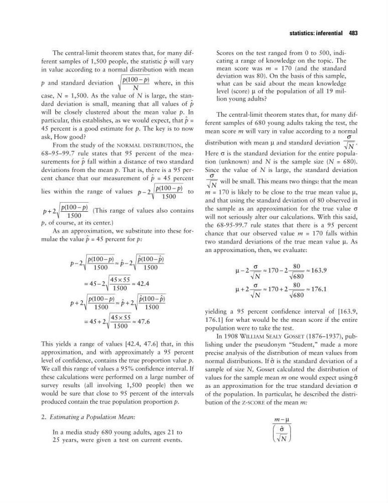
The central-limit theorem states that, for many different samples of 1,500 people, the statistic ˆ
p will vary
in value according to a normal distribution with mean
p and standard deviation
where, in this
case, N = 1,500. As the value of N is large, the standard deviation is small, meaning that all values of ˆ
p
will be closely clustered about the mean value p. In
particular, this establishes, as we would expect, that ˆ
p =
45 percent is a good estimate for p. The key is to now
ask, How good?
From the study of the NORMAL DISTRIBUTION, the
68–95–99.7 rule states that 95 percent of the measurements for ˆ
p fall within a distance of two standard
deviations from the mean p. That is, there is a 95 percent chance that our measurement of ˆ
p = 45 percent
lies within the range of values
to
(This range of values also contains
p, of course, at its center.)
As an approximation, we substitute into these formulae the value ˆ
p = 45 percent for p:
This yields a range of values [42.4, 47.6] that, in this
approximation, and with approximately a 95 percent
level of confidence, contains the true proportion value p.
We call this range of values a 95% confidence interval. If
these calculations were performed on a large number of
survey results (all involving 1,500 people) then we
would be sure that close to 95 percent of the intervals
produced contain the true population proportion p.
2. Estimating a Population Mean:
In a media study 680 young adults, ages 21 to
25 years, were given a test on current events.
Scores on the test ranged from 0 to 500, indicating a range of knowledge on the topic. The
mean score was m = 170 (and the standard
deviation was 80). On the basis of this sample,
what can be said about the mean knowledge
level (score) µ of the population of all 19 million young adults?
The central-limit theorem states that, for many different samples of 680 young adults taking the test, the
mean score m will vary in value according to a normal
distribution with mean µ and standard deviation
.
Here σ is the standard deviation for the entire population (unknown) and N is the sample size (N = 680).
Since the value of N is large, the standard deviation
will be small. This means two things: that the mean
m = 170 is likely to be close to the true mean value µ,
and that using the standard deviation of 80 observed in
the sample as an approximation for the true value σ
will not seriously alter our calculations. With this said,
the 68-95-99.7 rule states that there is a 95 percent
chance that our observed value m = 170 falls within
two standard deviations of the true mean value µ. As
an approximation, then, we evaluate:
yielding a 95 percent confidence interval of [163.9,
176.1] for what would be the mean score if the entire
population were to take the test.
In 1908 WILLIAM SEALY GOSSET (1876–1937), publishing under the pseudonym “Student,” made a more
precise analysis of the distribution of mean values from
normal distributions. If ˆ
σ is the standard deviation of a
sample of size N, Gosset calculated the distribution of
values for the sample mean m one would expect using ˆ
σ
as an approximation for the true standard deviation σ
of the population. In particular, he described the distribution of the Z-SCORE of the mean m:
m
N
−
µ
σ ˆ
µ
σ
µ
σ
−
≈
−
≈
+
≈
+
≈
2
170 2
80
680
163 9
2
170 2
80
680
176 1
N
N
.
.
σ
N
σ
N
p
p
p p
p
p
p
p
p p
p
p
−
− ≈ −
−
= −
×
≈
+
− ≈ +
−
=
+
×
≈
2
100
1500
2
100
1500
45 2
45 55
1500
42 4
2
100
1500
2
100
1500
45 2
45 55
1500
47 6
(
) ˆ
ˆ (
ˆ )
.
(
) ˆ
ˆ (
ˆ )
.
p
p
p
+
−
2
100
1500
(
)
p
p
p
−
−
2
100
1500
(
)
p
p
N
(
)
100 −
statistics: inferential 483
p will vary
in value according to a normal distribution with mean
p and standard deviation
where, in this
case, N = 1,500. As the value of N is large, the standard deviation is small, meaning that all values of ˆ
p
will be closely clustered about the mean value p. In
particular, this establishes, as we would expect, that ˆ
p =
45 percent is a good estimate for p. The key is to now
ask, How good?
From the study of the NORMAL DISTRIBUTION, the
68–95–99.7 rule states that 95 percent of the measurements for ˆ
p fall within a distance of two standard
deviations from the mean p. That is, there is a 95 percent chance that our measurement of ˆ
p = 45 percent
lies within the range of values
to
(This range of values also contains
p, of course, at its center.)
As an approximation, we substitute into these formulae the value ˆ
p = 45 percent for p:
This yields a range of values [42.4, 47.6] that, in this
approximation, and with approximately a 95 percent
level of confidence, contains the true proportion value p.
We call this range of values a 95% confidence interval. If
these calculations were performed on a large number of
survey results (all involving 1,500 people) then we
would be sure that close to 95 percent of the intervals
produced contain the true population proportion p.
2. Estimating a Population Mean:
In a media study 680 young adults, ages 21 to
25 years, were given a test on current events.
Scores on the test ranged from 0 to 500, indicating a range of knowledge on the topic. The
mean score was m = 170 (and the standard
deviation was 80). On the basis of this sample,
what can be said about the mean knowledge
level (score) µ of the population of all 19 million young adults?
The central-limit theorem states that, for many different samples of 680 young adults taking the test, the
mean score m will vary in value according to a normal
distribution with mean µ and standard deviation
.
Here σ is the standard deviation for the entire population (unknown) and N is the sample size (N = 680).
Since the value of N is large, the standard deviation
will be small. This means two things: that the mean
m = 170 is likely to be close to the true mean value µ,
and that using the standard deviation of 80 observed in
the sample as an approximation for the true value σ
will not seriously alter our calculations. With this said,
the 68-95-99.7 rule states that there is a 95 percent
chance that our observed value m = 170 falls within
two standard deviations of the true mean value µ. As
an approximation, then, we evaluate:
yielding a 95 percent confidence interval of [163.9,
176.1] for what would be the mean score if the entire
population were to take the test.
In 1908 WILLIAM SEALY GOSSET (1876–1937), publishing under the pseudonym “Student,” made a more
precise analysis of the distribution of mean values from
normal distributions. If ˆ
σ is the standard deviation of a
sample of size N, Gosset calculated the distribution of
values for the sample mean m one would expect using ˆ
σ
as an approximation for the true standard deviation σ
of the population. In particular, he described the distribution of the Z-SCORE of the mean m:
m
N
−
µ
σ ˆ
µ
σ
µ
σ
−
≈
−
≈
+
≈
+
≈
2
170 2
80
680
163 9
2
170 2
80
680
176 1
N
N
.
.
σ
N
σ
N
p
p
p p
p
p
p
p
p p
p
p
−
− ≈ −
−
= −
×
≈
+
− ≈ +
−
=
+
×
≈
2
100
1500
2
100
1500
45 2
45 55
1500
42 4
2
100
1500
2
100
1500
45 2
45 55
1500
47 6
(
) ˆ
ˆ (
ˆ )
.
(
) ˆ
ˆ (
ˆ )
.
p
p
p
+
−
2
100
1500
(
)
p
p
p
−
−
2
100
1500
(
)
p
p
N
(
)
100 −
statistics: inferential 483