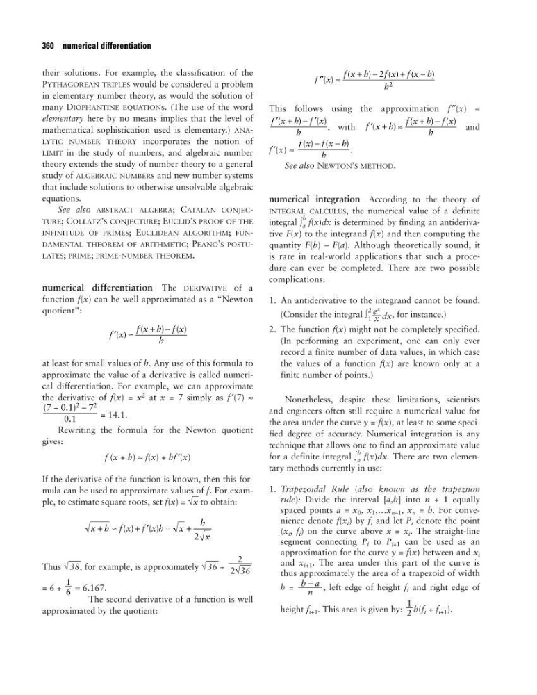
their solutions. For example, the classification of the
PYTHAGOREAN TRIPLES would be considered a problem
in elementary number theory, as would the solution of
many DIOPHANTINE EQUATIONs. (The use of the word
elementary here by no means implies that the level of
mathematical sophistication used is elementary.) ANALYTIC NUMBER THEORY incorporates the notion of
LIMIT in the study of numbers, and algebraic number
theory extends the study of number theory to a general
study of ALGEBRAIC NUMBERs and new number systems
that include solutions to otherwise unsolvable algebraic
equations.
See also ABSTRACT ALGEBRA; CATALAN CONJECTURE; COLLATZ’S CONJECTURE; EUCLID’S PROOF OF THE
INFINITUDE OF PRIMES; EUCLIDEAN ALGORITHM; FUNDAMENTAL THEOREM OF ARITHMETIC; PEANO’S POSTULATES; PRIME; PRIME-NUMBER THEOREM.
numerical differentiation The DERIVATIVE of a
function f(x) can be well approximated as a “Newton
quotient”:
at least for small values of h. Any use of this formula to
approximate the value of a derivative is called numerical differentiation. For example, we can approximate
the derivative of f(x) = x
2 at x = 7 simply as f ′(7) ≈
= 14.1.
Rewriting the formula for the Newton quotient
gives:
f (x + h) ≈ f(x) + hf ′(x)
If the derivative of the function is known, then this formula can be used to approximate values of f. For example, to estimate square roots, set f(x) = √
–
x to obtain:
Thus √
–
38, for example, is approximately √
–
36 +
= 6 +
≈ 6.167.
The second derivative of a function is well
approximated by the quotient:
This follows using the approximation f ″(x) ≈
, with
and
f ′(x) ≈
.
See also NEWTON’S METHOD.
numerical integration According to the theory of
INTEGRAL CALCULUS, the numerical value of a definite
integral ∫
b
a f(x)dx is determined by finding an antiderivative F(x) to the integrand f(x) and then computing the
quantity F(b) – F(a). Although theoretically sound, it
is rare in real-world applications that such a procedure can ever be completed. There are two possible
complications:
1. An antiderivative to the integrand cannot be found.
(Consider the integral ∫
2
1
dx , for instance.)
2. The function f(x) might not be completely specified.
(In performing an experiment, one can only ever
record a finite number of data values, in which case
the values of a function f(x) are known only at a
finite number of points.)
Nonetheless, despite these limitations, scientists
and engineers often still require a numerical value for
the area under the curve y = f(x), at least to some specified degree of accuracy. Numerical integration is any
technique that allows one to find an approximate value
for a definite integral ∫
b
a f(x)dx. There are two elementary methods currently in use:
1. Trapezoidal Rule (also known as the trapezium
rule): Divide the interval [a,b] into n + 1 equally
spaced points a = x 0 , x 1 ,…x n–1 , x n = b. For convenience denote f(x i ) by f i and let P i denote the point
(x i , f i ) on the curve above x = x i . The straight-line
segment connecting P i to P i+1 can be used as an
approximation for the curve y = f(x) between and x i
and x i+1 . The area under this part of the curve is
thus approximately the area of a trapezoid of width
h =
, left edge of height f i and right edge of
height f i+1 . This area is given by: h(f i + f i+1 ).
1
–
2
b – a
–––
n
e
x
– x
f x f x h
h
( ) (
)
−
−
′ + ≈
+ −
f x h
f x h f x
h
(
)
(
) ( )
′ + − ′
f x h f x
h
(
)
( )
′′ ≈
+ −
+
−
f x
f x h
f x f x h
h
( )
(
)
( ) (
)
2
2
1
–
6
2
–––
2√
–
36
x h f x f x h
x
h
x
+ ≈
+ ′
=
+
( )
( )
2
(7 + 0.1)
2 – 7
2
––––––––
0.1
′ ≈
+ −
f x
f x h f x
h
( )
(
) ( )
360 numerical differentiation