

tribution of mean zero and standard deviation 1 (the
standard normal distribution). One can convert an
arbitrary normal distribution into a standard normal
form by use of Z-SCOREs, which then allows one to
calculate probabilities for that distribution.
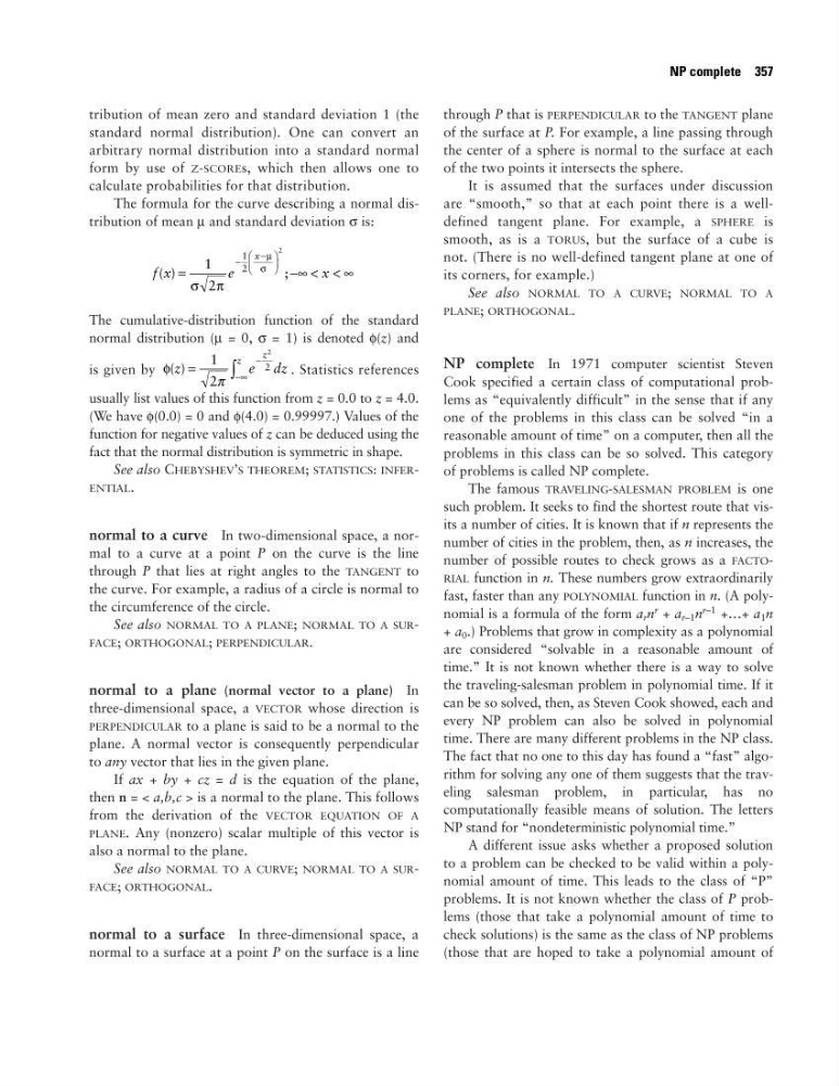
The formula for the curve describing a normal distribution of mean µ and standard deviation σ is:
The cumulative-distribution function of the standard
normal distribution (µ = 0, σ = 1) is denoted φ(z) and
is given by
. Statistics references
usually list values of this function from z = 0.0 to z = 4.0.
(We have φ(0.0) = 0 and φ(4.0) = 0.99997.) Values of the
function for negative values of z can be deduced using the
fact that the normal distribution is symmetric in shape.
See also CHEBYSHEV’S THEOREM; STATISTICS: INFERENTIAL.
normal to a curve In two-dimensional space, a normal to a curve at a point P on the curve is the line
through P that lies at right angles to the TANGENT to
the curve. For example, a radius of a circle is normal to
the circumference of the circle.
See also NORMAL TO A PLANE; NORMAL TO A SURFACE; ORTHOGONAL; PERPENDICULAR.
normal to a plane (normal vector to a plane) In
three-dimensional space, a VECTOR whose direction is
PERPENDICULAR to a plane is said to be a normal to the
plane. A normal vector is consequently perpendicular
to any vector that lies in the given plane.
If ax + by + cz = d is the equation of the plane,
then n = < a,b,c > is a normal to the plane. This follows
from the derivation of the VECTOR EQUATION OF A
PLANE. Any (nonzero) scalar multiple of this vector is
also a normal to the plane.
See also NORMAL TO A CURVE; NORMAL TO A SURFACE; ORTHOGONAL.
normal to a surface In three-dimensional space, a
normal to a surface at a point P on the surface is a line
through P that is PERPENDICULAR to the TANGENT plane
of the surface at P. For example, a line passing through
the center of a sphere is normal to the surface at each
of the two points it intersects the sphere.
It is assumed that the surfaces under discussion
are “smooth,” so that at each point there is a welldefined tangent plane. For example, a SPHERE is
smooth, as is a TORUS, but the surface of a cube is
not. (There is no well-defined tangent plane at one of
its corners, for example.)
See also NORMAL TO A CURVE; NORMAL TO A
PLANE; ORTHOGONAL.
NP complete In 1971 computer scientist Steven
Cook specified a certain class of computational problems as “equivalently difficult” in the sense that if any
one of the problems in this class can be solved “in a
reasonable amount of time” on a computer, then all the
problems in this class can be so solved. This category
of problems is called NP complete.
The famous TRAVELING-SALESMAN PROBLEM is one
such problem. It seeks to find the shortest route that visits a number of cities. It is known that if n represents the
number of cities in the problem, then, as n increases, the
number of possible routes to check grows as a FACTORIAL function in n. These numbers grow extraordinarily
fast, faster than any POLYNOMIAL function in n. (A polynomial is a formula of the form a r n
r + a r–1 n
r–1 +…+ a 1 n
+ a 0 .) Problems that grow in complexity as a polynomial
are considered “solvable in a reasonable amount of
time.” It is not known whether there is a way to solve
the traveling-salesman problem in polynomial time. If it
can be so solved, then, as Steven Cook showed, each and
every NP problem can also be solved in polynomial
time. There are many different problems in the NP class.
The fact that no one to this day has found a “fast” algorithm for solving any one of them suggests that the traveling salesman problem, in particular, has no
computationally feasible means of solution. The letters
NP stand for “nondeterministic polynomial time.”
A different issue asks whether a proposed solution
to a problem can be checked to be valid within a polynomial amount of time. This leads to the class of “P”
problems. It is not known whether the class of P problems (those that take a polynomial amount of time to
check solutions) is the same as the class of NP problems
(those that are hoped to take a polynomial amount of
φ( )
z
e d z
z
z
=
−
−∞
∫
1
2
2
2
π
f x
e
x
x
( )
;
=
− ∞ < < ∞
−
−
1
2
1
2
2
σ π
µ
σ
NP complete 357
standard normal distribution). One can convert an
arbitrary normal distribution into a standard normal
form by use of Z-SCOREs, which then allows one to
calculate probabilities for that distribution.
The formula for the curve describing a normal distribution of mean µ and standard deviation σ is:
The cumulative-distribution function of the standard
normal distribution (µ = 0, σ = 1) is denoted φ(z) and
is given by
. Statistics references
usually list values of this function from z = 0.0 to z = 4.0.
(We have φ(0.0) = 0 and φ(4.0) = 0.99997.) Values of the
function for negative values of z can be deduced using the
fact that the normal distribution is symmetric in shape.
See also CHEBYSHEV’S THEOREM; STATISTICS: INFERENTIAL.
normal to a curve In two-dimensional space, a normal to a curve at a point P on the curve is the line
through P that lies at right angles to the TANGENT to
the curve. For example, a radius of a circle is normal to
the circumference of the circle.
See also NORMAL TO A PLANE; NORMAL TO A SURFACE; ORTHOGONAL; PERPENDICULAR.
normal to a plane (normal vector to a plane) In
three-dimensional space, a VECTOR whose direction is
PERPENDICULAR to a plane is said to be a normal to the
plane. A normal vector is consequently perpendicular
to any vector that lies in the given plane.
If ax + by + cz = d is the equation of the plane,
then n = < a,b,c > is a normal to the plane. This follows
from the derivation of the VECTOR EQUATION OF A
PLANE. Any (nonzero) scalar multiple of this vector is
also a normal to the plane.
See also NORMAL TO A CURVE; NORMAL TO A SURFACE; ORTHOGONAL.
normal to a surface In three-dimensional space, a
normal to a surface at a point P on the surface is a line
through P that is PERPENDICULAR to the TANGENT plane
of the surface at P. For example, a line passing through
the center of a sphere is normal to the surface at each
of the two points it intersects the sphere.
It is assumed that the surfaces under discussion
are “smooth,” so that at each point there is a welldefined tangent plane. For example, a SPHERE is
smooth, as is a TORUS, but the surface of a cube is
not. (There is no well-defined tangent plane at one of
its corners, for example.)
See also NORMAL TO A CURVE; NORMAL TO A
PLANE; ORTHOGONAL.
NP complete In 1971 computer scientist Steven
Cook specified a certain class of computational problems as “equivalently difficult” in the sense that if any
one of the problems in this class can be solved “in a
reasonable amount of time” on a computer, then all the
problems in this class can be so solved. This category
of problems is called NP complete.
The famous TRAVELING-SALESMAN PROBLEM is one
such problem. It seeks to find the shortest route that visits a number of cities. It is known that if n represents the
number of cities in the problem, then, as n increases, the
number of possible routes to check grows as a FACTORIAL function in n. These numbers grow extraordinarily
fast, faster than any POLYNOMIAL function in n. (A polynomial is a formula of the form a r n
r + a r–1 n
r–1 +…+ a 1 n
+ a 0 .) Problems that grow in complexity as a polynomial
are considered “solvable in a reasonable amount of
time.” It is not known whether there is a way to solve
the traveling-salesman problem in polynomial time. If it
can be so solved, then, as Steven Cook showed, each and
every NP problem can also be solved in polynomial
time. There are many different problems in the NP class.
The fact that no one to this day has found a “fast” algorithm for solving any one of them suggests that the traveling salesman problem, in particular, has no
computationally feasible means of solution. The letters
NP stand for “nondeterministic polynomial time.”
A different issue asks whether a proposed solution
to a problem can be checked to be valid within a polynomial amount of time. This leads to the class of “P”
problems. It is not known whether the class of P problems (those that take a polynomial amount of time to
check solutions) is the same as the class of NP problems
(those that are hoped to take a polynomial amount of
φ( )
z
e d z
z
z
=
−
−∞
∫
1
2
2
2
π
f x
e
x
x
( )
;
=
− ∞ < < ∞
−
−
1
2
1
2
2
σ π
µ
σ
NP complete 357