

Despite the simplicity of the Riemannian model, it
was not immediately obvious to scholars of the 19th
century that it was permissible. Euclid’s second postulate seems to state that straight lines should be of infinite length. Riemann had the insight to note that
“extended indefinitely” does not imply “infinitely
long,” thus allowing him to consider a geometry in
which straight lines loop back on themselves.
In hyperbolic geometry, all angles in a triangle sum
to less than 180°, and the ratio of the circumference of
a circle to its diameter is greater than π. In spherical
geometry, all angles in a triangle sum to more than
180°, and the ratio of the circumference of a circle to
its diameter is less than π. EUCLIDEAN GEOMETRY, in
which angles in a triangle always sum exactly to 180°
and the ratio of the circumference to diameter of any
circle is precisely π, can thus be regarded as an intermediate between the two.
See also EUCLID; PLAYFAIR’S AXIOM.
normal distribution In the early 1700s scientists
noticed that errors from measurements in scientific
experiments repeated many times tended to follow the
same form of DISTRIBUTION, even though the studies
were conducted in unrelated fields (physics versus
biology or sociology, for example). The particular pattern of errors observed is today known as the normal
distribution (or Gaussian distribution). The French
mathematician ABRAHAM DE MOIVRE, in 1733, was
the first to write a mathematical formula for the distribution. Later, mathematicians PIERRE-SIMON LAPLACE
(1749–1827), SIMÉON-DENIS POISSON (1781–1840),
and CARL FRIEDRICH GAUSS (1777–1855) specified and
proved many of its mathematical properties. At the turn
of the 20th century Aleksandr Mikhailovich Lyapunov,
and later others, refined and developed Laplace’s work
to establish the CENTRAL-LIMIT THEOREM to explain the
frequent occurrence of the normal distribution in all scientific studies.
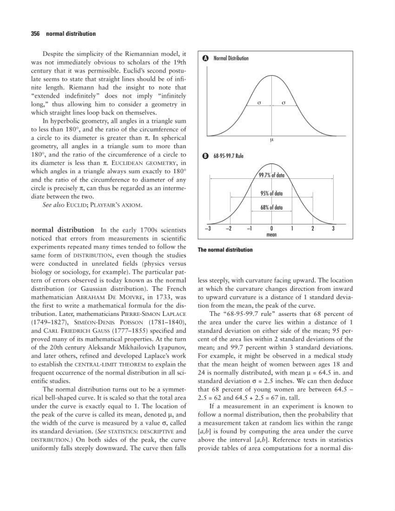
The normal distribution turns out to be a symmetrical bell-shaped curve. It is scaled so that the total area
under the curve is exactly equal to 1. The location of
the peak of the curve is called its mean, denoted µ, and
the width of the curve is measured by a value σ, called
its standard deviation. (See STATISTICS: DESCRIPTIVE and
DISTRIBUTION.) On both sides of the peak, the curve
uniformly falls steeply downward. The curve then falls
less steeply, with curvature facing upward. The location
at which the curvature changes direction from inward
to upward curvature is a distance of 1 standard deviation from the mean, the peak of the curve.
The “68-95-99.7 rule” asserts that 68 percent of
the area under the curve lies within a distance of 1
standard deviation on either side of the mean; 95 percent of the area lies within 2 standard deviations of the
mean; and 99.7 percent within 3 standard deviations.
For example, it might be observed in a medical study
that the mean height of women between ages 18 and
24 is normally distributed, with mean µ = 64.5 in. and
standard deviation σ = 2.5 inches. We can then deduce
that 68 percent of young women are between 64.5 –
2.5 = 62 and 64.5 + 2.5 = 67 in. tall.
If a measurement in an experiment is known to
follow a normal distribution, then the probability that
a measurement taken at random lies within the range
[a,b] is found by computing the area under the curve
above the interval [a,b]. Reference texts in statistics
provide tables of area computations for a normal dis356 normal distribution
The normal distribution
was not immediately obvious to scholars of the 19th
century that it was permissible. Euclid’s second postulate seems to state that straight lines should be of infinite length. Riemann had the insight to note that
“extended indefinitely” does not imply “infinitely
long,” thus allowing him to consider a geometry in
which straight lines loop back on themselves.
In hyperbolic geometry, all angles in a triangle sum
to less than 180°, and the ratio of the circumference of
a circle to its diameter is greater than π. In spherical
geometry, all angles in a triangle sum to more than
180°, and the ratio of the circumference of a circle to
its diameter is less than π. EUCLIDEAN GEOMETRY, in
which angles in a triangle always sum exactly to 180°
and the ratio of the circumference to diameter of any
circle is precisely π, can thus be regarded as an intermediate between the two.
See also EUCLID; PLAYFAIR’S AXIOM.
normal distribution In the early 1700s scientists
noticed that errors from measurements in scientific
experiments repeated many times tended to follow the
same form of DISTRIBUTION, even though the studies
were conducted in unrelated fields (physics versus
biology or sociology, for example). The particular pattern of errors observed is today known as the normal
distribution (or Gaussian distribution). The French
mathematician ABRAHAM DE MOIVRE, in 1733, was
the first to write a mathematical formula for the distribution. Later, mathematicians PIERRE-SIMON LAPLACE
(1749–1827), SIMÉON-DENIS POISSON (1781–1840),
and CARL FRIEDRICH GAUSS (1777–1855) specified and
proved many of its mathematical properties. At the turn
of the 20th century Aleksandr Mikhailovich Lyapunov,
and later others, refined and developed Laplace’s work
to establish the CENTRAL-LIMIT THEOREM to explain the
frequent occurrence of the normal distribution in all scientific studies.
The normal distribution turns out to be a symmetrical bell-shaped curve. It is scaled so that the total area
under the curve is exactly equal to 1. The location of
the peak of the curve is called its mean, denoted µ, and
the width of the curve is measured by a value σ, called
its standard deviation. (See STATISTICS: DESCRIPTIVE and
DISTRIBUTION.) On both sides of the peak, the curve
uniformly falls steeply downward. The curve then falls
less steeply, with curvature facing upward. The location
at which the curvature changes direction from inward
to upward curvature is a distance of 1 standard deviation from the mean, the peak of the curve.
The “68-95-99.7 rule” asserts that 68 percent of
the area under the curve lies within a distance of 1
standard deviation on either side of the mean; 95 percent of the area lies within 2 standard deviations of the
mean; and 99.7 percent within 3 standard deviations.
For example, it might be observed in a medical study
that the mean height of women between ages 18 and
24 is normally distributed, with mean µ = 64.5 in. and
standard deviation σ = 2.5 inches. We can then deduce
that 68 percent of young women are between 64.5 –
2.5 = 62 and 64.5 + 2.5 = 67 in. tall.
If a measurement in an experiment is known to
follow a normal distribution, then the probability that
a measurement taken at random lies within the range
[a,b] is found by computing the area under the curve
above the interval [a,b]. Reference texts in statistics
provide tables of area computations for a normal dis356 normal distribution
The normal distribution