

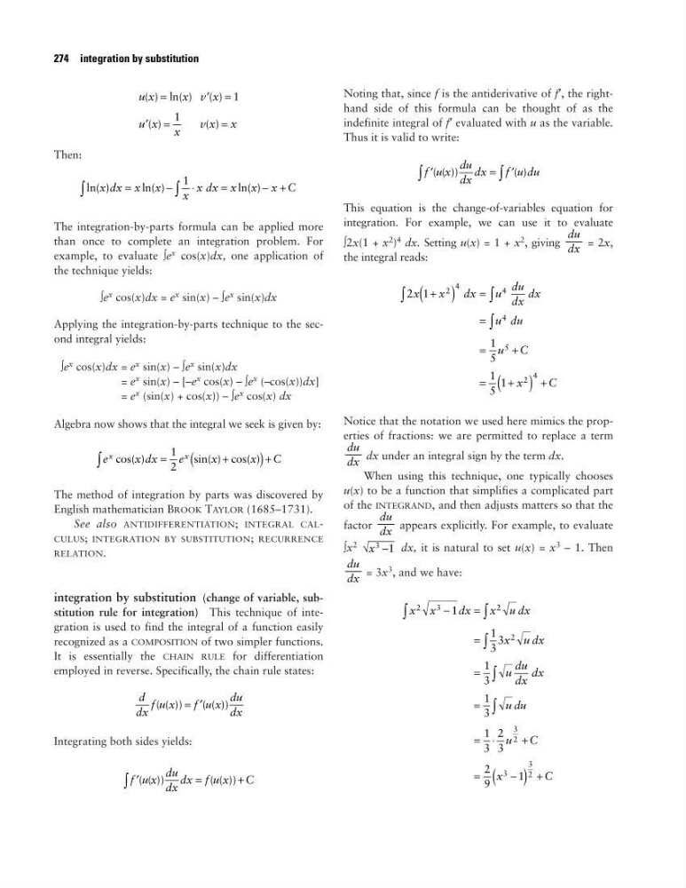
Then:
The integration-by-parts formula can be applied more
than once to complete an integration problem. For
example, to evaluate ∫e
x cos(x)dx, one application of
the technique yields:
∫e
x cos(x)dx = e
x sin(x) – ∫e
x sin(x)dx
Applying the integration-by-parts technique to the second integral yields:
∫e
x cos(x)dx = e
x sin(x) – ∫e
x sin(x)dx
= e
x sin(x) – [–e
x cos(x) – ∫e
x (–cos(x))dx]
= e
x (sin(x) + cos(x)) – ∫e
x cos(x) dx
Algebra now shows that the integral we seek is given by:
The method of integration by parts was discovered by
English mathematician BROOK TAYLOR (1685–1731).
See also ANTIDIFFERENTIATION; INTEGRAL CALCULUS; INTEGRATION BY SUBSTITUTION; RECURRENCE
RELATION.
integration by substitution (change of variable, substitution rule for integration) This technique of integration is used to find the integral of a function easily
recognized as a COMPOSITION of two simpler functions.
It is essentially the CHAIN RULE for differentiation
employed in reverse. Specifically, the chain rule states:
Integrating both sides yields:
Noting that, since f is the antiderivative of f′, the righthand side of this formula can be thought of as the
indefinite integral of f′ evaluated with u as the variable.
Thus it is valid to write:
This equation is the change-of-variables equation for
integration. For example, we can use it to evaluate
∫2x(1 + x
2
)
4 dx. Setting u(x) = 1 + x
2
, giving
= 2x,
the integral reads:
Notice that the notation we used here mimics the properties of fractions: we are permitted to replace a term
dx under an integral sign by the term dx.
When using this technique, one typically chooses
u(x) to be a function that simplifies a complicated part
of the INTEGRAND, and then adjusts matters so that the
factor
appears explicitly. For example, to evaluate
∫x
2
dx, it is natural to set u(x) = x
3 – 1. Then
= 3x
3
, and we have:
x x
dx
x u dx
x udx
u
du
dx
dx
u du
u
C
x
C
2
3
2
2
3
2
3
3
2
1
1
3
3
1
3
1
3
1
3
2
3
2
9
1
−
=
=
=
=
= ⋅
+
=
−
( ) +
∫
∫
∫
∫
∫
du
––
dx
√x
3 –1
du
––
dx
du
––
dx
2 1
1
5
1
5
1
2
4
4
4
5
2
4
x
x
dx
u
du
dx
dx
u du
u C
x
C
+
( ) =
=
=
+
=
+
( ) +
∫
∫
∫
du
––
dx
′
= ′
∫
∫
f u x
du
dx
dx
f u du
( ( ))
( )
′
=
+
∫ f u x
du
dx
dx f u x C
( ( ))
( ( ))
d
dx
f u x
f u x
du
dx
( ( ))
( ( ))
= ′
e
x dx
e
x
x C
x
x
cos( )
sin( ) cos( )
=
+
(
) +
∫
1
2
ln( )
ln( )
ln( )
x dx x x
x
x dx x x x C
=
−
⋅
=
− +
∫
∫
1
u x
x v x
u x x
v x x
( ) ln( )
( )
( )
( )
=
′ =
′ =
=
1
1
274 integration by substitution
The integration-by-parts formula can be applied more
than once to complete an integration problem. For
example, to evaluate ∫e
x cos(x)dx, one application of
the technique yields:
∫e
x cos(x)dx = e
x sin(x) – ∫e
x sin(x)dx
Applying the integration-by-parts technique to the second integral yields:
∫e
x cos(x)dx = e
x sin(x) – ∫e
x sin(x)dx
= e
x sin(x) – [–e
x cos(x) – ∫e
x (–cos(x))dx]
= e
x (sin(x) + cos(x)) – ∫e
x cos(x) dx
Algebra now shows that the integral we seek is given by:
The method of integration by parts was discovered by
English mathematician BROOK TAYLOR (1685–1731).
See also ANTIDIFFERENTIATION; INTEGRAL CALCULUS; INTEGRATION BY SUBSTITUTION; RECURRENCE
RELATION.
integration by substitution (change of variable, substitution rule for integration) This technique of integration is used to find the integral of a function easily
recognized as a COMPOSITION of two simpler functions.
It is essentially the CHAIN RULE for differentiation
employed in reverse. Specifically, the chain rule states:
Integrating both sides yields:
Noting that, since f is the antiderivative of f′, the righthand side of this formula can be thought of as the
indefinite integral of f′ evaluated with u as the variable.
Thus it is valid to write:
This equation is the change-of-variables equation for
integration. For example, we can use it to evaluate
∫2x(1 + x
2
)
4 dx. Setting u(x) = 1 + x
2
, giving
= 2x,
the integral reads:
Notice that the notation we used here mimics the properties of fractions: we are permitted to replace a term
dx under an integral sign by the term dx.
When using this technique, one typically chooses
u(x) to be a function that simplifies a complicated part
of the INTEGRAND, and then adjusts matters so that the
factor
appears explicitly. For example, to evaluate
∫x
2
dx, it is natural to set u(x) = x
3 – 1. Then
= 3x
3
, and we have:
x x
dx
x u dx
x udx
u
du
dx
dx
u du
u
C
x
C
2
3
2
2
3
2
3
3
2
1
1
3
3
1
3
1
3
1
3
2
3
2
9
1
−
=
=
=
=
= ⋅
+
=
−
( ) +
∫
∫
∫
∫
∫
du
––
dx
√x
3 –1
du
––
dx
du
––
dx
2 1
1
5
1
5
1
2
4
4
4
5
2
4
x
x
dx
u
du
dx
dx
u du
u C
x
C
+
( ) =
=
=
+
=
+
( ) +
∫
∫
∫
du
––
dx
′
= ′
∫
∫
f u x
du
dx
dx
f u du
( ( ))
( )
′
=
+
∫ f u x
du
dx
dx f u x C
( ( ))
( ( ))
d
dx
f u x
f u x
du
dx
( ( ))
( ( ))
= ′
e
x dx
e
x
x C
x
x
cos( )
sin( ) cos( )
=
+
(
) +
∫
1
2
ln( )
ln( )
ln( )
x dx x x
x
x dx x x x C
=
−
⋅
=
− +
∫
∫
1
u x
x v x
u x x
v x x
( ) ln( )
( )
( )
( )
=
′ =
′ =
=
1
1
274 integration by substitution