

An even better approximation could be made using
more points and consequently shorter line segments.
The actual length of the curve would be the LIMIT value
of these improved approximations as we use shorter
and shorter line segments connecting more and more
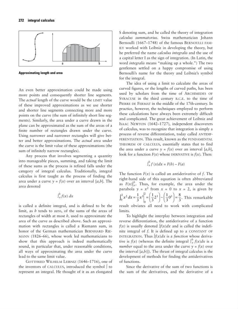
points on the curve (the sum of infinitely short line segments). Similarly, the area under a curve drawn in the
plane can be approximated as the sum of the areas of a
finite number of rectangles drawn under the curve.
Using narrower and narrower rectangles will give better and better approximations. The actual area under
the curve is the limit value of these approximations (the
sum of infinitely narrow rectangles).
Any process that involves segmenting a quantity
into manageable pieces, summing, and taking the limit
of these sums as the process is refined falls under the
category of integral calculus. Traditionally, integral
calculus is first taught as the process of finding the
area under a curve y = f(x) over an interval [a,b]. The
area denoted
∫
b
a f(x) dx
is called a definite integral, and is defined to be the
limit, as h tends to zero, of the sums of the areas of
rectangles of width at most h, used to approximate the
area of the curve as described above. Such an approximation with rectangles is called a Riemann sum, in
honor of the German mathematician BERNHARD RIEMANN (1826–66), whose work led mathematicians to
show that this approach is indeed mathematically
sound, in particular that, under reasonable conditions,
all ways of approximating the area under the curve
lead to the same limit value.
GOTTFRIED WILHELM LEIBNIZ (1646–1716), one of
the inventors of CALCULUS, introduced the symbol ∫ to
represent an integral. He thought of it as an elongated
S denoting sum, and he called the theory of integration
calculus summatorius. Swiss mathematician Johann
Bernoulli (1667–1748) of the famous BERNOULLI FAMILY worked with Leibniz in developing the theory, but
he preferred the name calculus integralis and the use of
a capital letter I as the sign of integration. (In Latin, the
word integralis means “making up a whole.”) The two
gentlemen settled on a happy compromise of using
Bernoulli’s name for the theory and Leibniz’s symbol
for the integral.
The idea of using a limit to calculate the areas of
curved figures, or the lengths of curved paths, has been
used by scholars from the time of ARCHIMEDES OF
SYRACUSE in the third century B.C.E. to the time of
PIERRE DE FERMAT in the middle of the 17th-century. In
practice, however, the techniques employed to perform
these calculations have always been extremely difficult
and complicated. The great achievement of Leibniz and
ISAAC NEWTON (1642–1727), independent discoverers
of calculus, was to recognize that integration is simply a
process of reverse differentiation, today called ANTIDIFFERENTIATION. This result, known as the FUNDAMENTAL
THEOREM OF CALCULUS, essentially states that to find
the area under a curve y = f(x) over an interval [a,b],
look for a function F(x) whose DERIVATIVE is f(x). Then:
∫
b
a f (x)dx = F(b) – F(a)
The function F(x) is called an antiderivative of f. The
right-hand side of this equation is often abbreviated
as F(x) |
b
a . Thus, for example, the area under the
parabola y = x
2 from x = 0 to x = 2, is given by
. This remarkable
result obviates all need to work with complicated
limits.
To highlight the interplay between integration and
reverse differentiation, the antiderivative of a function
f(x) is usually denoted ∫f(x)dx and is called the indefinite integral of f. It is defined up to a CONSTANT OF
INTEGRATION. Thus ∫f(x)dx is a function whose derivative is f(x) (whereas the definite integral ∫
b
a f(x)dx is a
number equal to the area under the curve y = f(x) over
the interval [a,b)]). The thrust of integral calculus is the
development of methods for finding the antiderivatives
of functions.
Since the derivative of the sum of two functions is
the sum of the derivatives, and the derivative of a
x dx
x
2
3
0
2
3
3
0
2
1
3
1
3
2
1
3
0
8
3
=
=
−
=
∫
272 integral calculus
Approximating length and area
more points and consequently shorter line segments.
The actual length of the curve would be the LIMIT value
of these improved approximations as we use shorter
and shorter line segments connecting more and more
points on the curve (the sum of infinitely short line segments). Similarly, the area under a curve drawn in the
plane can be approximated as the sum of the areas of a
finite number of rectangles drawn under the curve.
Using narrower and narrower rectangles will give better and better approximations. The actual area under
the curve is the limit value of these approximations (the
sum of infinitely narrow rectangles).
Any process that involves segmenting a quantity
into manageable pieces, summing, and taking the limit
of these sums as the process is refined falls under the
category of integral calculus. Traditionally, integral
calculus is first taught as the process of finding the
area under a curve y = f(x) over an interval [a,b]. The
area denoted
∫
b
a f(x) dx
is called a definite integral, and is defined to be the
limit, as h tends to zero, of the sums of the areas of
rectangles of width at most h, used to approximate the
area of the curve as described above. Such an approximation with rectangles is called a Riemann sum, in
honor of the German mathematician BERNHARD RIEMANN (1826–66), whose work led mathematicians to
show that this approach is indeed mathematically
sound, in particular that, under reasonable conditions,
all ways of approximating the area under the curve
lead to the same limit value.
GOTTFRIED WILHELM LEIBNIZ (1646–1716), one of
the inventors of CALCULUS, introduced the symbol ∫ to
represent an integral. He thought of it as an elongated
S denoting sum, and he called the theory of integration
calculus summatorius. Swiss mathematician Johann
Bernoulli (1667–1748) of the famous BERNOULLI FAMILY worked with Leibniz in developing the theory, but
he preferred the name calculus integralis and the use of
a capital letter I as the sign of integration. (In Latin, the
word integralis means “making up a whole.”) The two
gentlemen settled on a happy compromise of using
Bernoulli’s name for the theory and Leibniz’s symbol
for the integral.
The idea of using a limit to calculate the areas of
curved figures, or the lengths of curved paths, has been
used by scholars from the time of ARCHIMEDES OF
SYRACUSE in the third century B.C.E. to the time of
PIERRE DE FERMAT in the middle of the 17th-century. In
practice, however, the techniques employed to perform
these calculations have always been extremely difficult
and complicated. The great achievement of Leibniz and
ISAAC NEWTON (1642–1727), independent discoverers
of calculus, was to recognize that integration is simply a
process of reverse differentiation, today called ANTIDIFFERENTIATION. This result, known as the FUNDAMENTAL
THEOREM OF CALCULUS, essentially states that to find
the area under a curve y = f(x) over an interval [a,b],
look for a function F(x) whose DERIVATIVE is f(x). Then:
∫
b
a f (x)dx = F(b) – F(a)
The function F(x) is called an antiderivative of f. The
right-hand side of this equation is often abbreviated
as F(x) |
b
a . Thus, for example, the area under the
parabola y = x
2 from x = 0 to x = 2, is given by
. This remarkable
result obviates all need to work with complicated
limits.
To highlight the interplay between integration and
reverse differentiation, the antiderivative of a function
f(x) is usually denoted ∫f(x)dx and is called the indefinite integral of f. It is defined up to a CONSTANT OF
INTEGRATION. Thus ∫f(x)dx is a function whose derivative is f(x) (whereas the definite integral ∫
b
a f(x)dx is a
number equal to the area under the curve y = f(x) over
the interval [a,b)]). The thrust of integral calculus is the
development of methods for finding the antiderivatives
of functions.
Since the derivative of the sum of two functions is
the sum of the derivatives, and the derivative of a
x dx
x
2
3
0
2
3
3
0
2
1
3
1
3
2
1
3
0
8
3
=
=
−
=
∫
272 integral calculus
Approximating length and area