

recorded via a histogram. The categories considered are
conveniently chosen intervals of height ranges, such as
36.1–40.0 in., 40.1–44.0 in., and so on, for example.
If the DATA gathered is numerical and can adopt a
continuous array of values, including fractional values
(for example, height can adopt fractional values—48
3/4 in., or 52.837 in. are possible measurements), then
one can choose narrower and narrower interval ranges
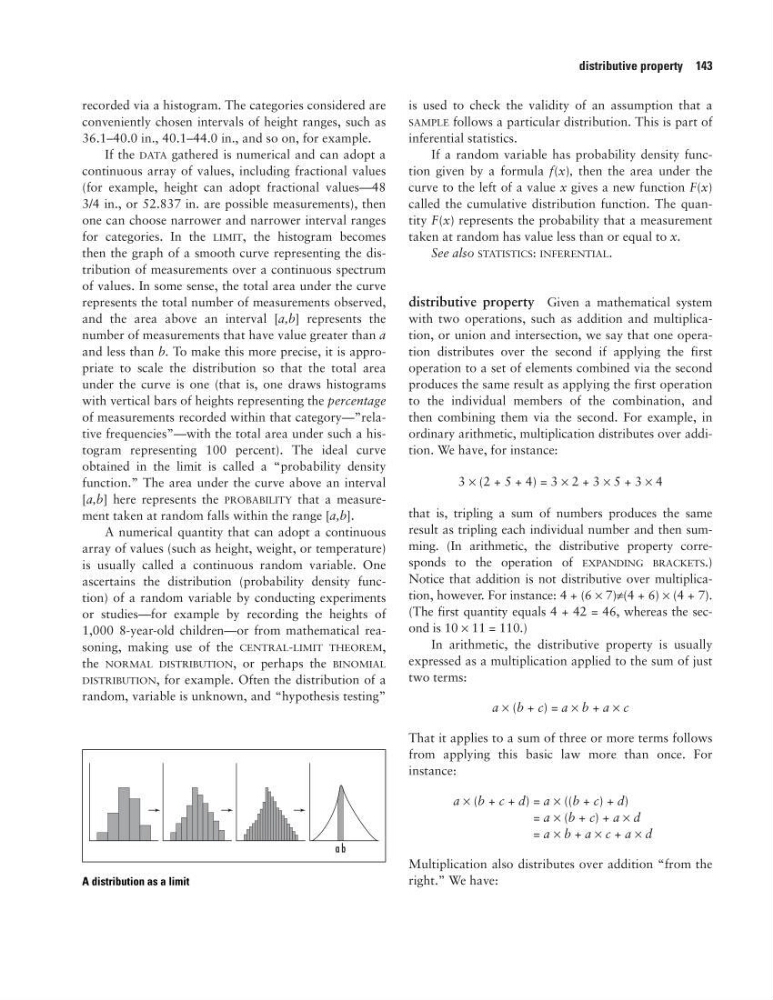
for categories. In the LIMIT, the histogram becomes
then the graph of a smooth curve representing the distribution of measurements over a continuous spectrum
of values. In some sense, the total area under the curve
represents the total number of measurements observed,
and the area above an interval [a,b] represents the
number of measurements that have value greater than a
and less than b. To make this more precise, it is appropriate to scale the distribution so that the total area
under the curve is one (that is, one draws histograms
with vertical bars of heights representing the percentage
of measurements recorded within that category—”relative frequencies”—with the total area under such a histogram representing 100 percent). The ideal curve
obtained in the limit is called a “probability density
function.” The area under the curve above an interval
[a,b] here represents the PROBABILITY that a measurement taken at random falls within the range [a,b].
A numerical quantity that can adopt a continuous
array of values (such as height, weight, or temperature)
is usually called a continuous random variable. One
ascertains the distribution (probability density function) of a random variable by conducting experiments
or studies—for example by recording the heights of
1,000 8-year-old children—or from mathematical reasoning, making use of the CENTRAL-LIMIT THEOREM,
the NORMAL DISTRIBUTION, or perhaps the BINOMIAL
DISTRIBUTION, for example. Often the distribution of a
random, variable is unknown, and “hypothesis testing”
is used to check the validity of an assumption that a
SAMPLE follows a particular distribution. This is part of
inferential statistics.
If a random variable has probability density function given by a formula f(x), then the area under the
curve to the left of a value x gives a new function F(x)
called the cumulative distribution function. The quantity F(x) represents the probability that a measurement
taken at random has value less than or equal to x.
See also STATISTICS: INFERENTIAL.
distributive property Given a mathematical system
with two operations, such as addition and multiplication, or union and intersection, we say that one operation distributes over the second if applying the first
operation to a set of elements combined via the second
produces the same result as applying the first operation
to the individual members of the combination, and
then combining them via the second. For example, in
ordinary arithmetic, multiplication distributes over addition. We have, for instance:
3 × (2 + 5 + 4) = 3 × 2 + 3 × 5 + 3 × 4
that is, tripling a sum of numbers produces the same
result as tripling each individual number and then summing. (In arithmetic, the distributive property corresponds to the operation of EXPANDING BRACKETS.)
Notice that addition is not distributive over multiplication, however. For instance: 4 + (6 × 7)≠(4 + 6) × (4 + 7).
(The first quantity equals 4 + 42 = 46, whereas the second is 10 × 11 = 110.)
In arithmetic, the distributive property is usually
expressed as a multiplication applied to the sum of just
two terms:
a × (b + c) = a × b + a × c
That it applies to a sum of three or more terms follows
from applying this basic law more than once. For
instance:
a × (b + c + d) = a × ((b + c) + d)
= a × (b + c) + a × d
= a × b + a × c + a × d
Multiplication also distributes over addition “from the
right.” We have:
distributive property 143
A distribution as a limit
conveniently chosen intervals of height ranges, such as
36.1–40.0 in., 40.1–44.0 in., and so on, for example.
If the DATA gathered is numerical and can adopt a
continuous array of values, including fractional values
(for example, height can adopt fractional values—48
3/4 in., or 52.837 in. are possible measurements), then
one can choose narrower and narrower interval ranges
for categories. In the LIMIT, the histogram becomes
then the graph of a smooth curve representing the distribution of measurements over a continuous spectrum
of values. In some sense, the total area under the curve
represents the total number of measurements observed,
and the area above an interval [a,b] represents the
number of measurements that have value greater than a
and less than b. To make this more precise, it is appropriate to scale the distribution so that the total area
under the curve is one (that is, one draws histograms
with vertical bars of heights representing the percentage
of measurements recorded within that category—”relative frequencies”—with the total area under such a histogram representing 100 percent). The ideal curve
obtained in the limit is called a “probability density
function.” The area under the curve above an interval
[a,b] here represents the PROBABILITY that a measurement taken at random falls within the range [a,b].
A numerical quantity that can adopt a continuous
array of values (such as height, weight, or temperature)
is usually called a continuous random variable. One
ascertains the distribution (probability density function) of a random variable by conducting experiments
or studies—for example by recording the heights of
1,000 8-year-old children—or from mathematical reasoning, making use of the CENTRAL-LIMIT THEOREM,
the NORMAL DISTRIBUTION, or perhaps the BINOMIAL
DISTRIBUTION, for example. Often the distribution of a
random, variable is unknown, and “hypothesis testing”
is used to check the validity of an assumption that a
SAMPLE follows a particular distribution. This is part of
inferential statistics.
If a random variable has probability density function given by a formula f(x), then the area under the
curve to the left of a value x gives a new function F(x)
called the cumulative distribution function. The quantity F(x) represents the probability that a measurement
taken at random has value less than or equal to x.
See also STATISTICS: INFERENTIAL.
distributive property Given a mathematical system
with two operations, such as addition and multiplication, or union and intersection, we say that one operation distributes over the second if applying the first
operation to a set of elements combined via the second
produces the same result as applying the first operation
to the individual members of the combination, and
then combining them via the second. For example, in
ordinary arithmetic, multiplication distributes over addition. We have, for instance:
3 × (2 + 5 + 4) = 3 × 2 + 3 × 5 + 3 × 4
that is, tripling a sum of numbers produces the same
result as tripling each individual number and then summing. (In arithmetic, the distributive property corresponds to the operation of EXPANDING BRACKETS.)
Notice that addition is not distributive over multiplication, however. For instance: 4 + (6 × 7)≠(4 + 6) × (4 + 7).
(The first quantity equals 4 + 42 = 46, whereas the second is 10 × 11 = 110.)
In arithmetic, the distributive property is usually
expressed as a multiplication applied to the sum of just
two terms:
a × (b + c) = a × b + a × c
That it applies to a sum of three or more terms follows
from applying this basic law more than once. For
instance:
a × (b + c + d) = a × ((b + c) + d)
= a × (b + c) + a × d
= a × b + a × c + a × d
Multiplication also distributes over addition “from the
right.” We have:
distributive property 143
A distribution as a limit