

Software Defined Security Monitoring in 5G Networks 241
In order to observe the whole system automatically, it is possible to have a Monitoring
Service (based, i.e. on Suricata [9] or MMT [10]), which communicates with the
Neutron and TaaS APIs. This service will observe and compare the ports of OpenStack
via Neutron API and analyze the traffic going through the ports that are mirrored by
the TaaS via the TaaS API. If a new virtual machine is created, a new port will be also
created, then the service will create a mirroring service for that port by using the TaaS
API. The Monitoring Service can be also implemented directly in a dedicated monitoring virtual machine, which helps simplify the deployment of the Monitoring Service in
OpenStack. This technique allows monitoring of all the traffic, but then a major issue
is scalability.
From the experiences gained from LTE monitoring, LTE control plane traffic of 2M
subscribers is approximately 300 Mbps/300 Kpps when S1‐MME, S6a and S11 interfaces are monitored. When using Intel DPDK, poll mode drivers capture to memory
is not a problem. DPDK optimized packet capture is capable of millions of PPS. In‐
house tests show that an SW analyser is able to perform 300 Mbps analysis with
6 cores at 3 GHz, with 64 GB of maximum amount of memory required and even DPI
type analysis of 10 Gbps of traffic is also possible using 16 cores (2.4 Mpps, where
packets have average size equal to 600 bytes). Similar results using Suricata can be
found in [13].
On the other hand, capture to disk is used to store raw packets for drilldown to be
used in troubleshooting. Capture to disk performance depends on the virtual storage.
The virtual storage must be selected to fulfil throughput and capacity requirements
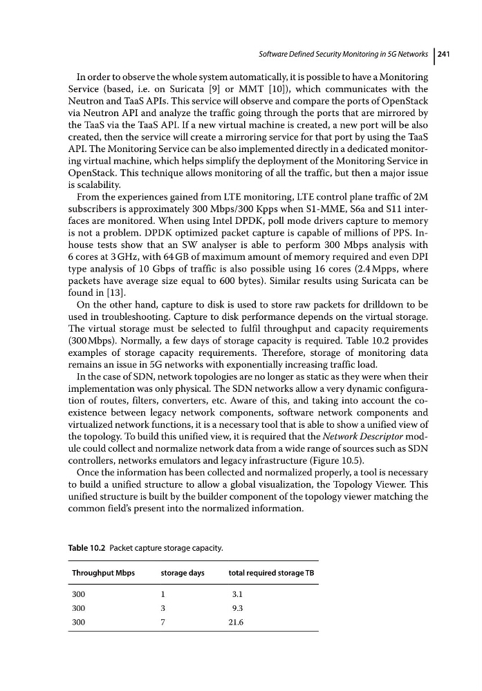
(300 Mbps). Normally, a few days of storage capacity is required. Table 10.2 provides
examples of storage capacity requirements. Therefore, storage of monitoring data
remains an issue in 5G networks with exponentially increasing traffic load.
In the case of SDN, network topologies are no longer as static as they were when their
implementation was only physical. The SDN networks allow a very dynamic configuration of routes, filters, converters, etc. Aware of this, and taking into account the co‐
existence between legacy network components, software network components and
virtualized network functions, it is a necessary tool that is able to show a unified view of
the topology. To build this unified view, it is required that the Network Descriptor module could collect and normalize network data from a wide range of sources such as SDN
controllers, networks emulators and legacy infrastructure (Figure 10.5).
Once the information has been collected and normalized properly, a tool is necessary
to build a unified structure to allow a global visualization, the Topology Viewer. This
unified structure is built by the builder component of the topology viewer matching the
common field’s present into the normalized information.
Table 10.2 Packet capture storage capacity.
Throughput Mbps
storage days
total required storage TB
300
1
3.1
300
3
9.3
300
7
21.6
In order to observe the whole system automatically, it is possible to have a Monitoring
Service (based, i.e. on Suricata [9] or MMT [10]), which communicates with the
Neutron and TaaS APIs. This service will observe and compare the ports of OpenStack
via Neutron API and analyze the traffic going through the ports that are mirrored by
the TaaS via the TaaS API. If a new virtual machine is created, a new port will be also
created, then the service will create a mirroring service for that port by using the TaaS
API. The Monitoring Service can be also implemented directly in a dedicated monitoring virtual machine, which helps simplify the deployment of the Monitoring Service in
OpenStack. This technique allows monitoring of all the traffic, but then a major issue
is scalability.
From the experiences gained from LTE monitoring, LTE control plane traffic of 2M
subscribers is approximately 300 Mbps/300 Kpps when S1‐MME, S6a and S11 interfaces are monitored. When using Intel DPDK, poll mode drivers capture to memory
is not a problem. DPDK optimized packet capture is capable of millions of PPS. In‐
house tests show that an SW analyser is able to perform 300 Mbps analysis with
6 cores at 3 GHz, with 64 GB of maximum amount of memory required and even DPI
type analysis of 10 Gbps of traffic is also possible using 16 cores (2.4 Mpps, where
packets have average size equal to 600 bytes). Similar results using Suricata can be
found in [13].
On the other hand, capture to disk is used to store raw packets for drilldown to be
used in troubleshooting. Capture to disk performance depends on the virtual storage.
The virtual storage must be selected to fulfil throughput and capacity requirements
(300 Mbps). Normally, a few days of storage capacity is required. Table 10.2 provides
examples of storage capacity requirements. Therefore, storage of monitoring data
remains an issue in 5G networks with exponentially increasing traffic load.
In the case of SDN, network topologies are no longer as static as they were when their
implementation was only physical. The SDN networks allow a very dynamic configuration of routes, filters, converters, etc. Aware of this, and taking into account the co‐
existence between legacy network components, software network components and
virtualized network functions, it is a necessary tool that is able to show a unified view of
the topology. To build this unified view, it is required that the Network Descriptor module could collect and normalize network data from a wide range of sources such as SDN
controllers, networks emulators and legacy infrastructure (Figure 10.5).
Once the information has been collected and normalized properly, a tool is necessary
to build a unified structure to allow a global visualization, the Topology Viewer. This
unified structure is built by the builder component of the topology viewer matching the
common field’s present into the normalized information.
Table 10.2 Packet capture storage capacity.
Throughput Mbps
storage days
total required storage TB
300
1
3.1
300
3
9.3
300
7
21.6