

90
For the development of the distribution maps, the kriging method with linear
variogram interpolation was applied. As area limits, we considered the percentile
values of the distribution of the interpolated values. The following seven areas of
percentile values were selected: 0–10, 10–25, 25–40, 40–60, 60–75, 75–90 and
90–100. The distribution maps for the individual elements are prepared in seven
concentration ranges for each element with different colour.
Factor 1 (Fe, Al, V, Ni, Li, Cr, Co, Ba, Pb, Sr and Mn) The spatial distribution
map of the factor scores of factor F1 (Fig. 3.5) shows that these elements are present
in varying concentrations throughout the studied area. Higher contents of these elements are found in the soil samples from the central part of the study where
Quaternary sediments are dominant geological formations as well as on the mountain Baba where Paleozoic schist and granites prevailed (Fig. 3.5). From the list of
the elements, it could be expected that some of the elements associated in Factor 1
have higher content in the area close to TEP Bitola and in the area between TEP
Bitola and the city of Bitola. This is visible from the maps of spatial distribution of
all elements included in Factor 1 which are presented in Fig. 3.6a and 3.6b. This
particularly applies to the spatial distribution of chromium (Fig. 3.6a) and zinc
(included in Factor 2) (Figs. 3.7 and 3.8) which are present in higher content in fly
ash than in the surrounding soil.
Factor 2 (Cu, Mo, Ag and Zn) The spatial distribution map of the factor scores of
factor F2 (Fig. 3.7) shows that these elements are present in higher contents in the
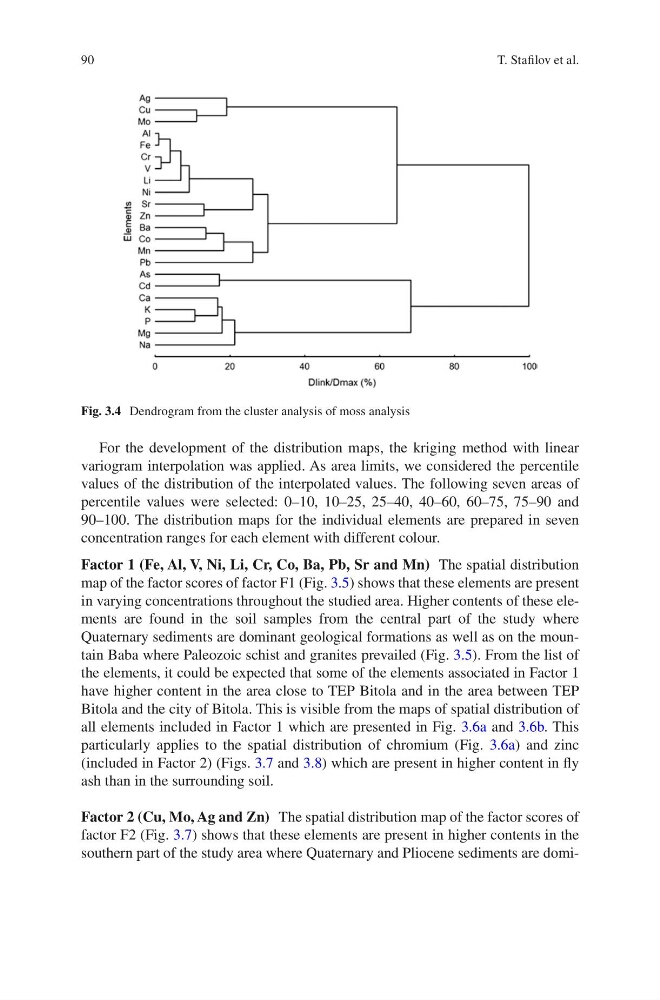
southern part of the study area where Quaternary and Pliocene sediments are domiFig. 3.4 Dendrogram from the cluster analysis of moss analysis
T. Stafilov et al.
For the development of the distribution maps, the kriging method with linear
variogram interpolation was applied. As area limits, we considered the percentile
values of the distribution of the interpolated values. The following seven areas of
percentile values were selected: 0–10, 10–25, 25–40, 40–60, 60–75, 75–90 and
90–100. The distribution maps for the individual elements are prepared in seven
concentration ranges for each element with different colour.
Factor 1 (Fe, Al, V, Ni, Li, Cr, Co, Ba, Pb, Sr and Mn) The spatial distribution
map of the factor scores of factor F1 (Fig. 3.5) shows that these elements are present
in varying concentrations throughout the studied area. Higher contents of these elements are found in the soil samples from the central part of the study where
Quaternary sediments are dominant geological formations as well as on the mountain Baba where Paleozoic schist and granites prevailed (Fig. 3.5). From the list of
the elements, it could be expected that some of the elements associated in Factor 1
have higher content in the area close to TEP Bitola and in the area between TEP
Bitola and the city of Bitola. This is visible from the maps of spatial distribution of
all elements included in Factor 1 which are presented in Fig. 3.6a and 3.6b. This
particularly applies to the spatial distribution of chromium (Fig. 3.6a) and zinc
(included in Factor 2) (Figs. 3.7 and 3.8) which are present in higher content in fly
ash than in the surrounding soil.
Factor 2 (Cu, Mo, Ag and Zn) The spatial distribution map of the factor scores of
factor F2 (Fig. 3.7) shows that these elements are present in higher contents in the
southern part of the study area where Quaternary and Pliocene sediments are domiFig. 3.4 Dendrogram from the cluster analysis of moss analysis
T. Stafilov et al.